Advancing your Search Engine

Why this lesson matters

In Introducing Search Engine, we built the core search primitive: a tokenization pipeline, an inverted index, full-text lookup, and a first ranking pass.

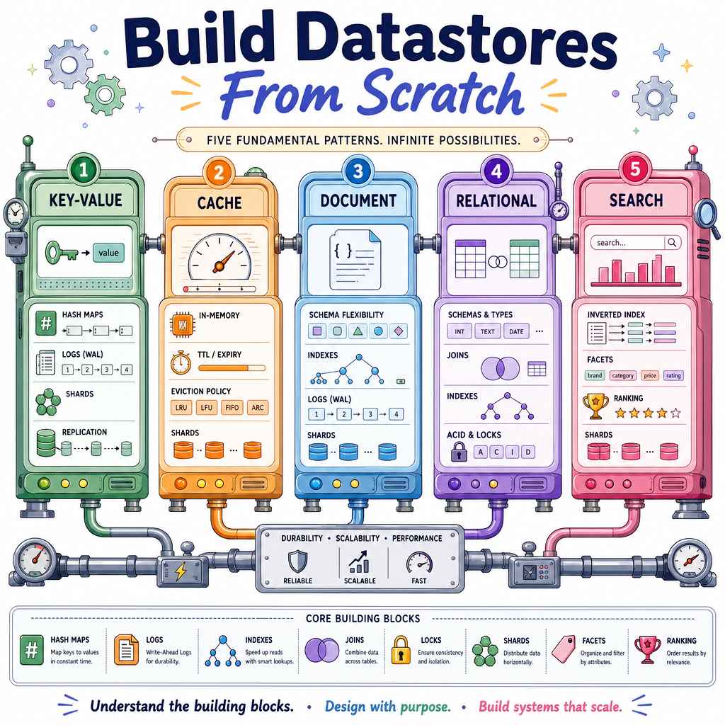
Now we finish the course by pushing that tiny engine closer to systems like Elasticsearch and OpenSearch:

• Distributed search: split work across shards, then merge results.
• Faceted search: return both matching documents and useful aggregations.
• Relevance scoring: rank results with a more principled scoring model.

This lesson also ties together patterns from earlier datastore builds: key-value lookup, document filtering, indexing, query planning, and tradeoffs around speed, consistency, and correctness.

One index becomes many shards

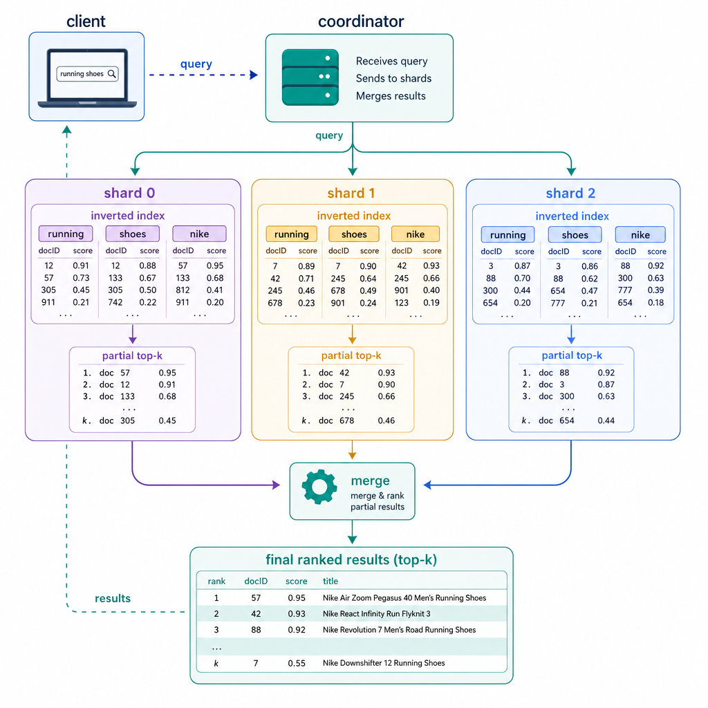
A production search engine usually does not keep one giant inverted index on one machine. It splits documents across shards.

A query then follows a coordinator pattern:

client query
    |
    v
coordinator
  /   |   \
shard shard shard
  \   |   /
    merge
    |
 ranked results

Each shard owns a subset of documents and can search locally. The coordinator asks every relevant shard for its top results, then merges those partial answers.

This should feel familiar from earlier lessons:

• From the key-value store lessons: route keys to storage locations.
• From the document database lessons: use indexes to avoid scanning everything.
• From the relational lessons: coordinate operators into a query plan.

The new twist is that search ranking makes merging trickier: each shard may have its own local statistics, so scores need careful normalization in real systems.

A tiny distributed search simulation

Below is not networked code, but it models the core idea: documents are assigned to shards, each shard builds its own inverted index, and a coordinator merges shard-local matches.

This is the same basic strategy used by large search systems, except real engines add replication, timeouts, retries, compression, caching, and cluster membership.

```python
import re
from collections import defaultdict


def tokenize(text):
    return re.findall(r"[a-z0-9]+", text.lower())


class Shard:
    def __init__(self, shard_id):
        self.shard_id = shard_id
        self.docs = {}
        self.index = defaultdict(set)

    def add(self, doc_id, text):
        self.docs[doc_id] = text
        for token in set(tokenize(text)):
            self.index[token].add(doc_id)

    def search(self, query):
        terms = tokenize(query)
        if not terms:
            return []

        matching = None
        for term in terms:
            ids = self.index.get(term, set())
            matching = ids if matching is None else matching & ids

        return sorted(matching or [])


class Coordinator:
    def __init__(self, shard_count):
        self.shards = [Shard(i) for i in range(shard_count)]

    def _pick_shard(self, doc_id):
        return doc_id % len(self.shards)

    def add(self, doc_id, text):
        self.shards[self._pick_shard(doc_id)].add(doc_id, text)

    def search(self, query):
        merged = []
        for shard in self.shards:
            local_hits = shard.search(query)
            print(f"shard {shard.shard_id} returned {local_hits}")
            merged.extend(local_hits)
        return sorted(merged)


engine = Coordinator(shard_count=3)
engine.add(1, "Python search engine internals")
engine.add(2, "Distributed systems and search clusters")
engine.add(3, "Finance news search and risk analytics")
engine.add(4, "Python indexing for document search")

print("Final results:", engine.search("python search"))
```

A search coordinator sends a query to several shards and receives each shard's local top results.

What is the coordinator's main responsibility next?

Search plus counts

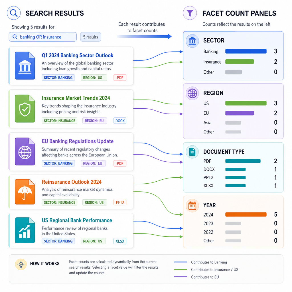
Faceted search answers two questions at once:

1. Which documents match?
2. How are those matches distributed across useful fields?

For example, a finance search for risk might return documents and also show:

sector
  banking: 2
  insurance: 1

region
  US: 2
  EU: 1

This is a natural extension of the document database work. In Enhancing your Document-Oriented Database, we used field indexes to narrow queries. Facets are similar, but instead of only filtering by fields, we also count field values among the matched documents.

In real products, facets power filters like category, brand, price range, author, exchange, rating, date, and region.

Counting fields over hits

A minimal faceted search engine can be built in three steps:

1. Search the inverted index to get matching document IDs.
2. Look up the original documents for those IDs.
3. Count selected metadata fields across the hits.

Notice the boundary: the inverted index finds text matches, while document metadata powers the facet counts.

```python
import re
from collections import defaultdict, Counter


def tokenize(text):
    return re.findall(r"[a-z0-9]+", text.lower())


class FacetedSearch:
    def __init__(self):
        self.docs = {}
        self.index = defaultdict(set)

    def add(self, doc_id, doc):
        self.docs[doc_id] = doc
        searchable_text = doc["title"] + " " + doc["body"]
        for token in set(tokenize(searchable_text)):
            self.index[token].add(doc_id)

    def search(self, query, facet_fields):
        terms = tokenize(query)
        hits = None
        for term in terms:
            ids = self.index.get(term, set())
            hits = ids if hits is None else hits & ids

        hits = sorted(hits or [])
        facets = {field: Counter() for field in facet_fields}

        for doc_id in hits:
            doc = self.docs[doc_id]
            for field in facet_fields:
                facets[field][doc.get(field, "unknown")] += 1

        return hits, facets


engine = FacetedSearch()
engine.add(1, {"title": "Bank risk report", "body": "Credit risk rising", "sector": "banking", "region": "US"})
engine.add(2, {"title": "Insurance risk model", "body": "Climate risk analysis", "sector": "insurance", "region": "EU"})
engine.add(3, {"title": "Bank earnings", "body": "Search demand and risk notes", "sector": "banking", "region": "US"})
engine.add(4, {"title": "Retail outlook", "body": "Consumer spending update", "sector": "retail", "region": "US"})

hits, facets = engine.search("risk", ["sector", "region"])
print("hits:", hits)
print("sector facets:", dict(facets["sector"]))
print("region facets:", dict(facets["region"]))
```

True or false: faceted search counts metadata values only across the documents that matched the current query, not necessarily across the entire corpus.

Better than boolean matching

In Introducing Search Engine, we ranked results enough to make search feel useful. Now we make that idea more explicit.

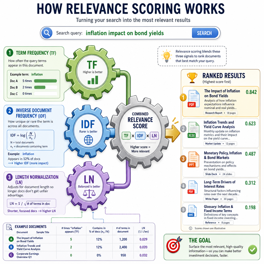
A classic relevance score asks:

• Does the document contain the query terms?
• How often do those terms appear in the document?
• Are those terms rare across the corpus?
• Is the document unusually long, making matches less impressive?

A common family of algorithms, including BM25, combines these ideas:

score = term frequency signal
      * inverse document frequency signal
      * document length normalization

For example, if the query is market risk, the word risk might appear in many finance documents, while volatility or liquidity may be more discriminating in a different query. Rarer terms often carry more ranking power.

A compact relevance algorithm

This example implements a small BM25-inspired scorer. It is not production-grade, but it captures the central intuition:

• More query term occurrences can help.
• Rare terms help more than common terms.
• Very long documents should not win just because they contain more words overall.

This is where search differs sharply from the earlier datastores: a key-value store returns a value, a relational database returns rows satisfying predicates, but a search engine returns a ranked judgment.

```python
import math
import re
from collections import Counter, defaultdict


def tokenize(text):
    return re.findall(r"[a-z0-9]+", text.lower())


class RankedSearch:
    def __init__(self):
        self.docs = {}
        self.term_freqs = {}
        self.postings = defaultdict(set)
        self.lengths = {}

    def add(self, doc_id, text):
        terms = tokenize(text)
        counts = Counter(terms)
        self.docs[doc_id] = text
        self.term_freqs[doc_id] = counts
        self.lengths[doc_id] = len(terms)
        for term in counts:
            self.postings[term].add(doc_id)

    def search(self, query, k=3, b=0.75, k1=1.5):
        query_terms = tokenize(query)
        n_docs = len(self.docs)
        avg_len = sum(self.lengths.values()) / max(n_docs, 1)
        scores = Counter()

        for term in query_terms:
            doc_ids = self.postings.get(term, set())
            if not doc_ids:
                continue

            # Smooth IDF so rare terms score higher without division-by-zero issues.
            idf = math.log(1 + (n_docs - len(doc_ids) + 0.5) / (len(doc_ids) + 0.5))

            for doc_id in doc_ids:
                tf = self.term_freqs[doc_id][term]
                doc_len = self.lengths[doc_id]
                denom = tf + k1 * (1 - b + b * doc_len / avg_len)
                scores[doc_id] += idf * ((tf * (k1 + 1)) / denom)

        return scores.most_common(k)


engine = RankedSearch()
engine.add(1, "python search engine indexing relevance")
engine.add(2, "python python python tutorial")
engine.add(3, "distributed search engine relevance scoring")
engine.add(4, "finance market risk search relevance")

for doc_id, score in engine.search("search relevance"):
    print(doc_id, round(score, 3), "->", engine.docs[doc_id])
```

In BM25-style ranking, the component that gives more weight to terms that appear in fewer documents is called inverse document ________.

What you built from scratch

You started with the datastore contract in Data Store Fundamentals and repeatedly asked: what does this system promise, and what data structures make those promises practical?

Across the course, you built primitive versions of:

• A key-value store with command semantics and expiration.
• A cache-like store with TTL and LRU behavior.
• A document database with matching and field indexes.
• A relational system with relations, joins, transactions, WAL, and locks.
• A search engine with tokenization, inverted indexes, ranking, shards, facets, and relevance.

The big lesson is not that these few Python classes replace PostgreSQL, Redis, MongoDB, or Elasticsearch. They do not.

The big lesson is that serious datastores are built from understandable pieces: maps, logs, indexes, counters, locks, query operators, and scoring functions. Once you can see those pieces, production systems become less magical and much easier to reason about.