Implementing Dynamic Linear Regression Models

Why this lesson matters

In Converting Second-Level Data to Time Frame Averages, you built the important trading object: one shared row that can hold features like a 30-minute moving average and a 60-minute moving average at the same timestamp.

Now we make that row useful for prediction.

A dynamic linear regression model answers:

Given the current feature row, what does the model expect next?

We are not wiring the model into the live WebSocket loop yet. That comes next in Integrating Predictions into the Dynamic Environment. Here, we focus on the model lifecycle itself:

feature row -> training matrix -> regression coefficients -> prediction

For an R workflow, this maps naturally to lm() and predict(). The runnable examples here use Python, but the data contract is the same.

Regression needs a label

Your moving averages are features. Linear regression also needs a target, sometimes called y.

For live trading, a common target is not raw price. Raw price is often non-stationary and scale-dependent. A cleaner beginner target is usually a future return:

target_next_return = close[t + 1] / close[t] - 1

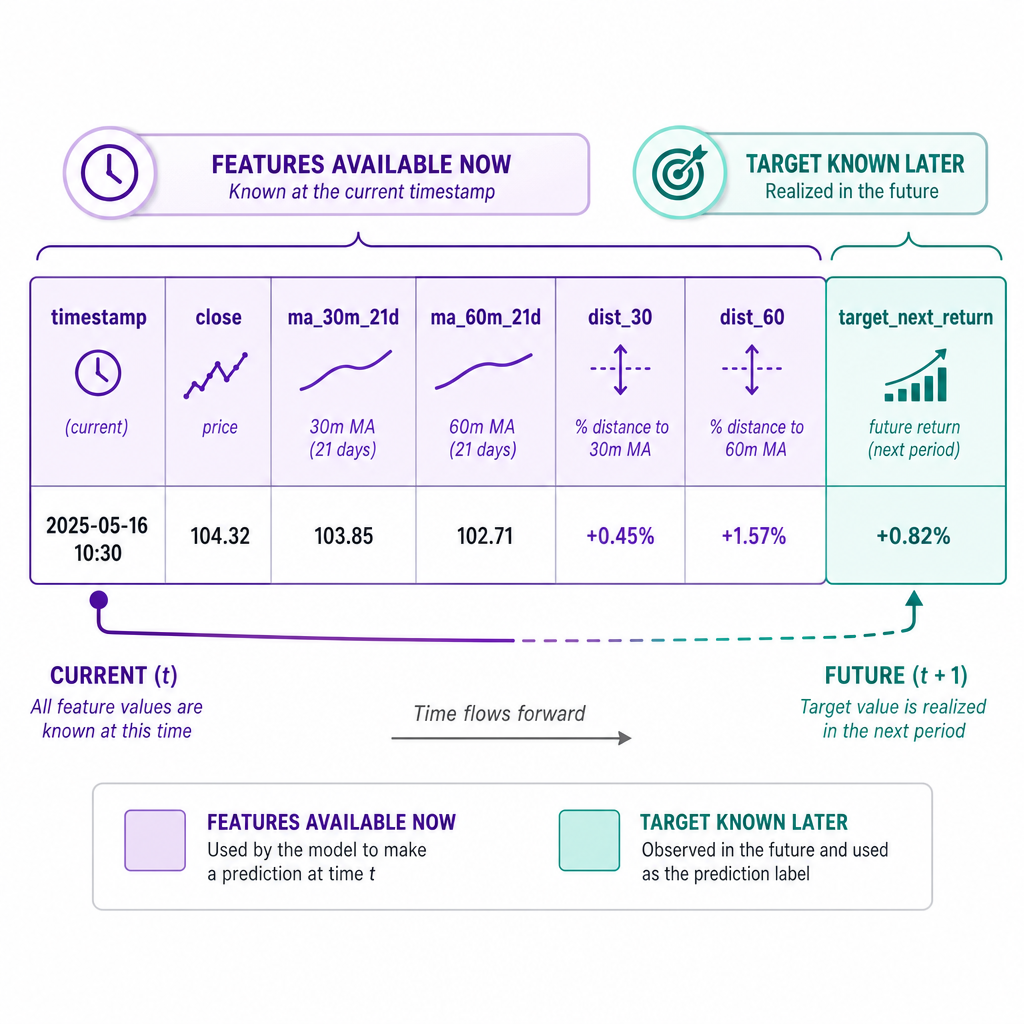
Then your row can look like:

timestamp | close | ma_30m_21d | ma_60m_21d | dist_30 | dist_60 | target_next_return

Where:

• dist_30 = close / ma_30m_21d - 1
• dist_60 = close / ma_60m_21d - 1
• target_next_return is known only after the next bar completes

This separation is critical. Features must be available at decision time. The label is only used for training after it becomes known.

Start with one historical snapshot

Before making anything dynamic, verify the model works on a completed feature table.

This example creates a miniature version of the row structure from the prior lesson, builds two moving-average distance features, and fits a linear regression with ordinary least squares.

The model form is:

next_return = b0 + b1 * dist_30 + b2 * dist_60

In R, this would be similar to:

lm(target_next_return ~ dist_30 + dist_60, data = train_df)

```python
import numpy as np
import pandas as pd

np.random.seed(7)

# Synthetic completed feature table: imagine this came from your 30m/60m aggregators.
n = 300
idx = pd.date_range('2024-01-01 09:30:00', periods=n, freq='30min')
returns = np.random.normal(0, 0.0015, n)
close = 100 * np.cumprod(1 + returns)

df = pd.DataFrame({'timestamp': idx, 'close': close})
df['ma_30m_21d'] = df['close'].rolling(42, min_periods=42).mean()
df['ma_60m_21d'] = df['close'].rolling(84, min_periods=84).mean()
df['dist_30'] = df['close'] / df['ma_30m_21d'] - 1
df['dist_60'] = df['close'] / df['ma_60m_21d'] - 1

# Target: the next row's return. This is shifted backward for supervised learning.
df['target_next_return'] = df['close'].shift(-1) / df['close'] - 1

model_df = df.dropna(subset=['dist_30', 'dist_60', 'target_next_return']).copy()

X = model_df[['dist_30', 'dist_60']].to_numpy()
y = model_df['target_next_return'].to_numpy()

# Add intercept column.
X_design = np.column_stack([np.ones(len(X)), X])
beta = np.linalg.lstsq(X_design, y, rcond=None)[0]

latest_features = X[-1]
latest_design = np.array([1, latest_features[0], latest_features[1]])
pred = latest_design @ beta

print('Rows used:', len(model_df))
print('Intercept:', round(beta[0], 8))
print('dist_30 coefficient:', round(beta[1], 6))
print('dist_60 coefficient:', round(beta[2], 6))
print('Latest predicted next return:', round(pred, 8))
```

You are processing a row at timestamp t and want to predict the next return after t.

Which value is safe to use as a feature at timestamp t?

Make the model dynamic

A static regression uses one fixed training table. A dynamic regression repeatedly refits as new labeled rows become available.

The key timing rule is:

At row t:
  train on rows whose targets are already known
  predict using features from row t

A common live approximation is a rolling window:

• Keep the most recent N labeled rows
• Refit the regression on that window
• Predict the next return for the current feature row

This lets the model adapt when market behavior changes, while avoiding using very old data forever.

```python
import numpy as np
import pandas as pd

np.random.seed(11)

n = 220
idx = pd.date_range('2024-02-01 09:30:00', periods=n, freq='30min')
returns = np.random.normal(0, 0.0012, n)
close = 50 * np.cumprod(1 + returns)

df = pd.DataFrame({'timestamp': idx, 'close': close})
df['ma_30m_21d'] = df['close'].rolling(30, min_periods=30).mean()
df['ma_60m_21d'] = df['close'].rolling(60, min_periods=60).mean()
df['dist_30'] = df['close'] / df['ma_30m_21d'] - 1
df['dist_60'] = df['close'] / df['ma_60m_21d'] - 1
df['target_next_return'] = df['close'].shift(-1) / df['close'] - 1

data = df.dropna(subset=['dist_30', 'dist_60', 'target_next_return']).reset_index(drop=True)
window = 80
predictions = []

for t in range(window, len(data)):
    train = data.iloc[t-window:t]
    current = data.iloc[t]

    X_train = train[['dist_30', 'dist_60']].to_numpy()
    y_train = train['target_next_return'].to_numpy()
    X_design = np.column_stack([np.ones(len(X_train)), X_train])

    beta = np.linalg.lstsq(X_design, y_train, rcond=None)[0]

    x_now = np.array([1, current['dist_30'], current['dist_60']])
    pred = float(x_now @ beta)

    predictions.append((current['timestamp'], pred))

print('Number of rolling predictions:', len(predictions))
print('First five predictions:')
for ts, pred in predictions[:5]:
    print(ts, 'predicted_next_return=', round(pred, 8))
```

True or false:

A dynamic regression model can safely train on the current row's target before predicting from that same row.

Keep model state separate

In Real-time Data Handling with WebSockets in R, you separated ingestion from live state. Do the same with modeling.

Your regression object should know how to:

• Store recent labeled examples
• Refit when enough data exists
• Predict from a new feature row
• Return None or skip prediction when undertrained

This keeps the model testable. The stream should not contain regression math scattered everywhere.

```python
import numpy as np
from collections import deque

class DynamicLinearRegression:
    def __init__(self, window=5, min_rows=3):
        self.window = window
        self.min_rows = min_rows
        self.examples = deque(maxlen=window)
        self.beta = None

    def add_labeled_row(self, features, target):
        self.examples.append((np.array(features, dtype=float), float(target)))
        self._fit_if_ready()

    def _fit_if_ready(self):
        if len(self.examples) < self.min_rows:
            self.beta = None
            return

        X = np.array([row[0] for row in self.examples])
        y = np.array([row[1] for row in self.examples])
        X_design = np.column_stack([np.ones(len(X)), X])
        self.beta = np.linalg.lstsq(X_design, y, rcond=None)[0]

    def predict(self, features):
        if self.beta is None:
            return None
        x = np.array([1, *features], dtype=float)
        return float(x @ self.beta)

model = DynamicLinearRegression(window=5, min_rows=3)

labeled_rows = [
    ([0.010, 0.006], 0.0007),
    ([0.005, 0.002], 0.0002),
    ([-0.004, -0.003], -0.0003),
    ([0.012, 0.007], 0.0008),
]

for features, target in labeled_rows:
    model.add_labeled_row(features, target)
    print('Rows stored:', len(model.examples), 'beta ready:', model.beta is not None)

current_features = [0.008, 0.004]
print('Prediction for current row:', round(model.predict(current_features), 8))
print('Current coefficients:', [round(x, 6) for x in model.beta])
```

Fill in the blank:

In the model

next_return = b0 + b1 * dist_30 + b2 * dist_60

b0 is the model's ______ term.

Regression output is not magic

A linear regression model gives you coefficients. For trading, coefficients are useful only if you interpret them cautiously.

Example:

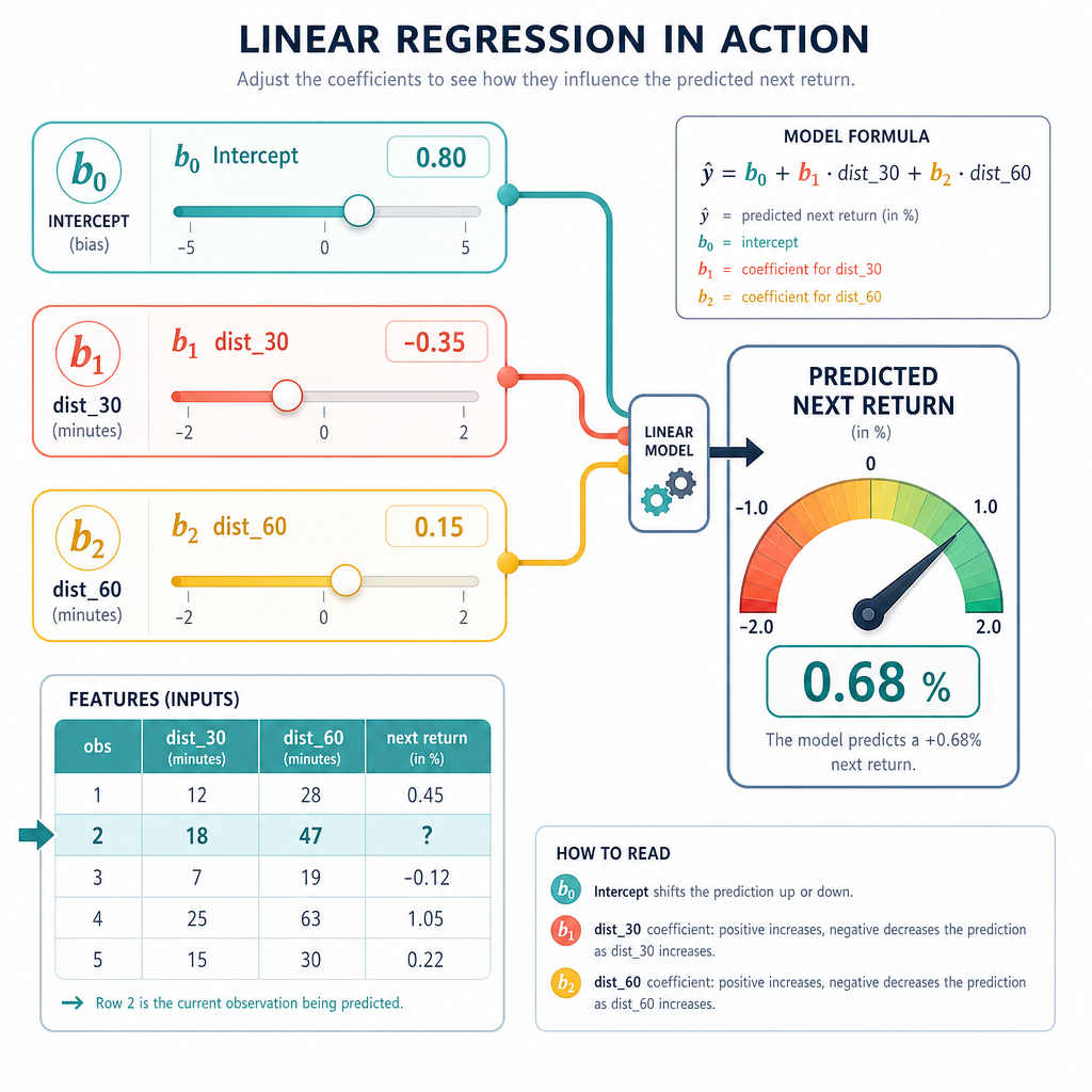
next_return = b0 + b1 * dist_30 + b2 * dist_60

If b1 is positive, the fitted model says that, within the training window, being farther above the 30-minute moving average was associated with a higher next return. That does not prove the relationship will continue.

In a live algo context, monitor:

• Prediction size: are predictions near zero or meaningful?
• Coefficient stability: do signs flip constantly?
• Training window size: too short can overfit, too long can go stale
• Feature scaling: distances are usually better than raw prices
• Out-of-sample behavior: live predictions matter more than in-sample fit

The model is a scoring component, not a trading system by itself.

What you now have

You can now turn the shared feature row from the previous lesson into a supervised learning row:

features now + target later -> labeled example

You also have the core pieces of a dynamic regression model:

• A feature matrix built from moving-average calculations
• A future-return target aligned without leakage
• A rolling refit process
• A small model state object with add_labeled_row() and predict() behavior

The next lesson connects this model to the live environment: when to update the model, when to call prediction, and how to attach the prediction back onto the same live row without turning the stream into a tangled script.