Integrating Predictions into the Dynamic Environment

Why this lesson matters

You have already built the pieces:

• Fetching OHLC Data from APIs gave us historical snapshots.
• Real-time Data Handling with WebSockets in R gave us live events.
• Converting Second-Level Data to Time Frame Averages turned seconds into shared 30/60-minute feature rows.
• Implementing Dynamic Linear Regression Models gave us a rolling model state.

Now we connect the final wire: each completed feature row enters a prediction function, receives a forecast, and becomes usable by a live decision layer.

The goal is not to make a profitable strategy here. The goal is to make the live architecture understandable and safe.

Where prediction lives

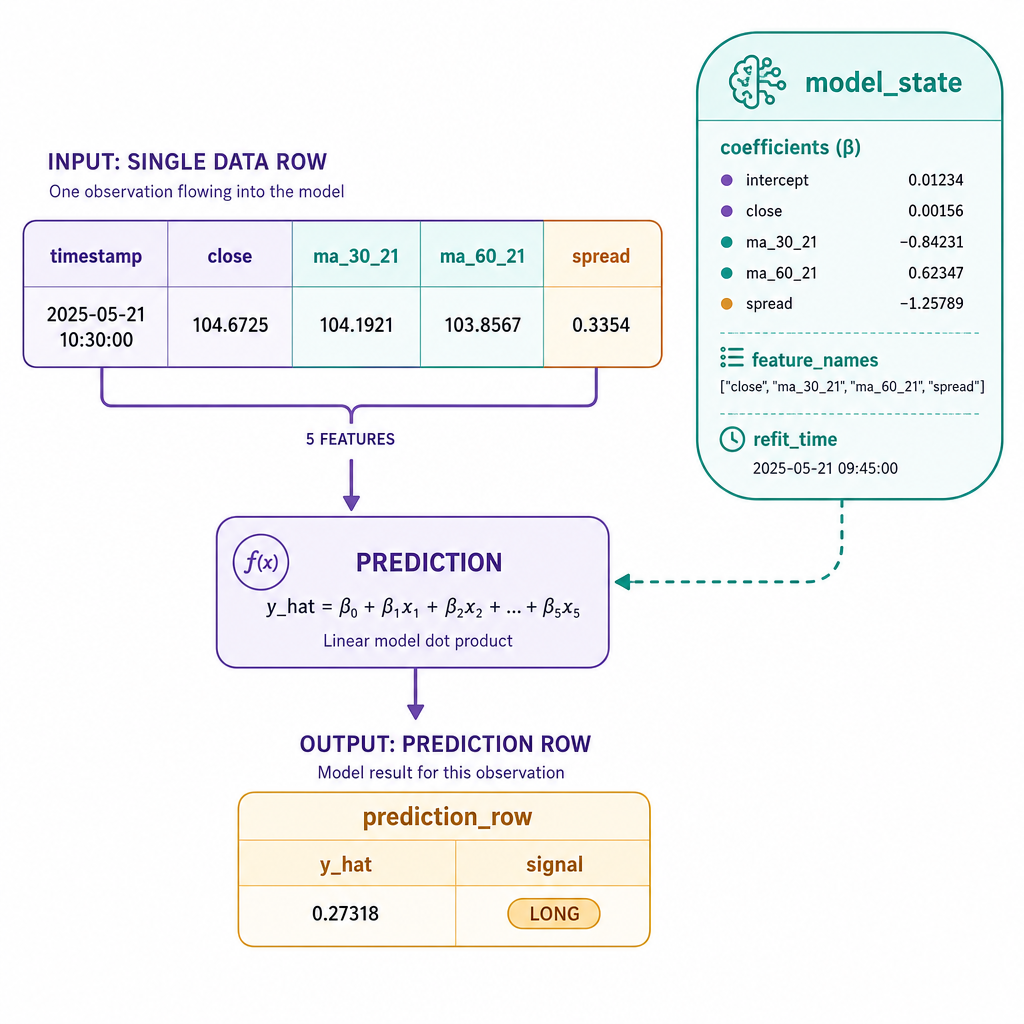
In the live loop, prediction is not a separate research notebook step. It is a small, repeatable operation:

completed shared row + current model_state -> prediction row

A prediction row usually contains:

• timestamp of the completed row
• features, such as ma_30_21, ma_60_21, and spread
• model version or refit time
• predicted value, such as next-period return
• signal-ready metadata, such as whether the row is complete

The key idea from One Shared Row still holds: the 30-minute and 60-minute calculations must be aligned to the same decision timestamp before the model sees them.

A compact dynamic example

The example below simulates minute closes, builds 30-minute and 60-minute 21-period moving averages, trains a rolling one-feature linear regression, and prints recent live-style predictions.

This mirrors the structure you would use with real API/WebSocket data: the data source changes, but the state machine stays familiar.

```python
from collections import deque
from datetime import datetime, timedelta
import math

# Deterministic synthetic minute close.
def price_at(minute):
    trend = 0.01 * minute
    cycle = 2.0 * math.sin(minute / 80.0)
    noise_like = 0.4 * math.sin(minute / 9.0)
    return 100 + trend + cycle + noise_like

def fit_ols(xs, ys):
    n = len(xs)
    x_bar = sum(xs) / n
    y_bar = sum(ys) / n
    denom = sum((x - x_bar) ** 2 for x in xs)
    if denom == 0:
        return {'intercept': y_bar, 'slope': 0.0}
    slope = sum((x - x_bar) * (y - y_bar) for x, y in zip(xs, ys)) / denom
    intercept = y_bar - slope * x_bar
    return {'intercept': intercept, 'slope': slope}

def predict(model, x):
    return model['intercept'] + model['slope'] * x

start = datetime(2025, 1, 1, 9, 30)
bar30_closes = deque(maxlen=21)
bar60_closes = deque(maxlen=21)
examples = []
prev_feature = None
prev_close = None
model = None
predictions = []

# Simulate enough minutes to create 21 sixty-minute bars plus training examples.
for minute in range(1, 3001):
    close = price_at(minute)

    if minute % 30 == 0:
        bar30_closes.append(close)

    if minute % 60 == 0:
        bar60_closes.append(close)
        ts = start + timedelta(minutes=minute)

        if len(bar30_closes) == 21 and len(bar60_closes) == 21:
            ma30_21 = sum(bar30_closes) / 21
            ma60_21 = sum(bar60_closes) / 21
            spread = ma30_21 - ma60_21

            # Now that current close is known, we can label the previous row.
            if prev_feature is not None:
                next_60m_change = close - prev_close
                examples.append((prev_feature, next_60m_change))

            # Refit from recent completed examples only.
            if len(examples) >= 20:
                recent = examples[-100:]
                xs = [x for x, y in recent]
                ys = [y for x, y in recent]
                model = fit_ols(xs, ys)
                y_hat = predict(model, spread)

                predictions.append({
                    'time': ts.strftime('%Y-%m-%d %H:%M'),
                    'ma30_21': round(ma30_21, 4),
                    'ma60_21': round(ma60_21, 4),
                    'spread': round(spread, 4),
                    'pred_next_60m_change': round(y_hat, 4)
                })

            prev_feature = spread
            prev_close = close

print('training_examples:', len(examples))
print('latest_model:', {k: round(v, 6) for k, v in model.items()})
print('recent_predictions:')
for row in predictions[-5:]:
    print(row)
```

A live prediction function should receive which input?

The prediction timing contract

Before a prediction is allowed, answer three questions:

1. Is the row complete?
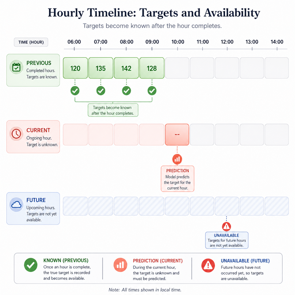
   Do not predict from a half-built 60-minute bar unless your strategy explicitly uses partial bars.

2. Is the model trained on only known targets?
   The previous row can be labeled once the next close exists. The current row cannot use its own future.

3. Is the model fresh enough?
   A model refit every row, every N rows, or every clock interval is fine. But the prediction row should record which model version produced it.

A practical live row often includes fields like:

row_time, ma_30_21, ma_60_21, spread, model_refit_time, y_hat

True or false: In a live system, it is safe to update the model with the current row's future return before making the current row's prediction.

Prediction is not yet an order

A model output is just a number. A signal layer turns that number into something operational.

For example:

• positive prediction above a threshold -> consider long
• negative prediction below a threshold -> consider short
• tiny prediction -> hold
• stale or incomplete row -> hold

This separation matters. You can improve the model without rewriting execution rules, and you can improve risk checks without retraining the model.

```python
def make_signal(row, threshold=0.15, max_model_age_minutes=180):
    if not row['is_complete']:
        return 'HOLD_incomplete_row'
    if row['model_age_minutes'] > max_model_age_minutes:
        return 'HOLD_stale_model'

    y_hat = row['pred_next_60m_change']
    trend_agrees_long = row['ma30_21'] > row['ma60_21']
    trend_agrees_short = row['ma30_21'] < row['ma60_21']

    if y_hat > threshold and trend_agrees_long:
        return 'BUY_candidate'
    if y_hat < -threshold and trend_agrees_short:
        return 'SELL_candidate'
    return 'HOLD_no_edge'

rows = [
    {'time': '2025-01-03 10:30', 'ma30_21': 112.4, 'ma60_21': 111.9, 'pred_next_60m_change': 0.31, 'model_age_minutes': 60, 'is_complete': True},
    {'time': '2025-01-03 11:30', 'ma30_21': 112.1, 'ma60_21': 112.3, 'pred_next_60m_change': -0.24, 'model_age_minutes': 60, 'is_complete': True},
    {'time': '2025-01-03 12:30', 'ma30_21': 112.2, 'ma60_21': 112.0, 'pred_next_60m_change': 0.05, 'model_age_minutes': 60, 'is_complete': True},
    {'time': '2025-01-03 13:30', 'ma30_21': 112.8, 'ma60_21': 112.2, 'pred_next_60m_change': 0.40, 'model_age_minutes': 240, 'is_complete': True}
]

for row in rows:
    print(row['time'], make_signal(row))
```

In this architecture, fitted coefficients, feature names, training window size, and last refit time should live inside ______.

What keeps this usable live

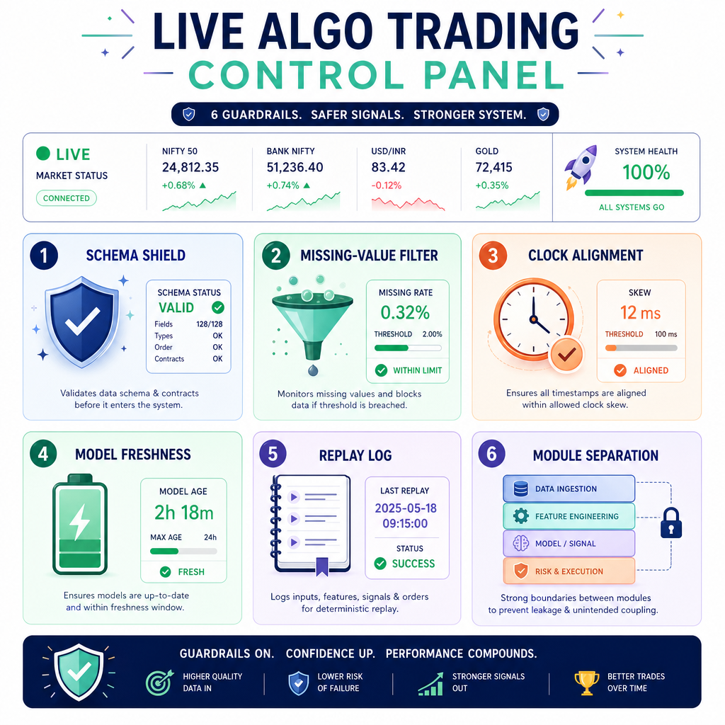
Once prediction is integrated, the fragile parts are usually not the regression formula. They are the live-system boundaries.

Add guardrails around:

• Schema: required fields exist before prediction.
• Missing values: do not silently predict from NA, NaN, or incomplete moving averages.
• Clock alignment: the 30-minute and 60-minute values must represent the same decision time.
• Model freshness: stale models should produce hold, not accidental trades.
• Replay logs: save enough rows to reproduce a prediction later.
• Separation: ingestion, aggregation, modeling, signal, and execution should remain separate modules.

This is how a small learning system starts to look like a real algo workflow.

The full mental model

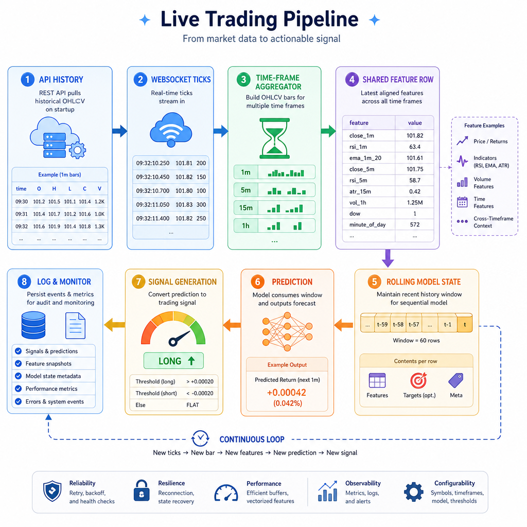
You can now describe the live pipeline end to end:

historical API seed
  -> WebSocket events
  -> normalized second-level rows
  -> 30/60-minute feature aggregation
  -> shared feature row
  -> rolling model_state
  -> prediction row
  -> signal layer
  -> logs and risk checks

The most important habit is to treat every update as an event that changes state in a controlled way.

In R, the same design maps naturally to data.table, xts, R6 objects, environments, or plain lists. In Python, the same design maps to dictionaries, classes, pandas objects, or queues. The language is less important than the contract between each stage.

You now have the foundation to turn second-level data into multi-timeframe features and live predictions without mixing research shortcuts into the dynamic environment.