Introduction to Quantum Computing

Why this lesson matters

Now that we've covered Introduction to Data Science, you've seen how Python can help us explore data, model uncertainty, and make careful predictions.

Quantum computing also deals with uncertainty—but in a very different way. Instead of uncertainty coming from incomplete data, quantum uncertainty is built into how information is represented and transformed.

In this lesson, you'll learn the core mental model:

• A bit is either 0 or 1.
• A qubit is described by amplitudes for 0 and 1.
• Quantum gates transform those amplitudes.
• Measurement turns quantum state into classical output.

We'll keep this practical and Python-focused, using small simulations rather than relying on a quantum SDK.

Classical bits

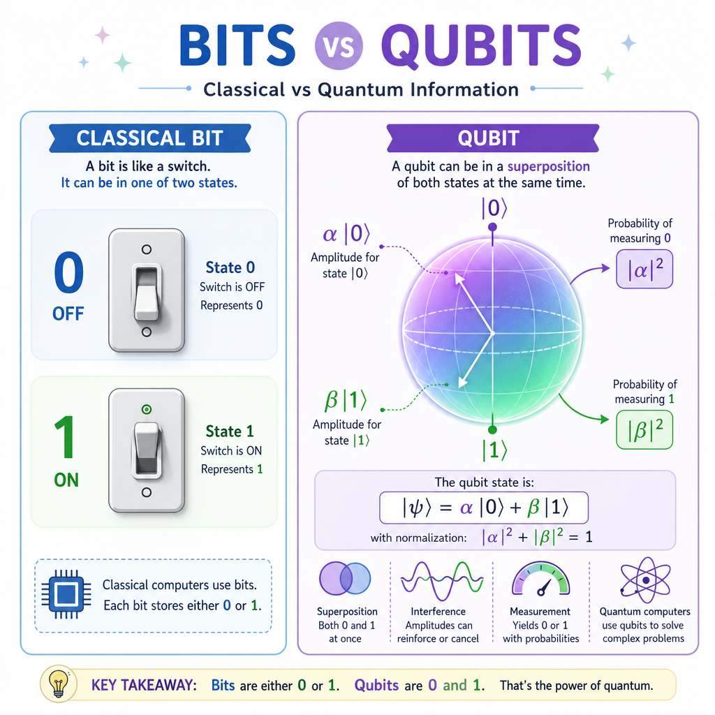
A classical bit has one definite value:

bit = 0
# or
bit = 1

This is the foundation of the systems you're already familiar with: web apps, databases, APIs, Angular state, C# backend logic, and normal Python programs.

Qubits

A qubit is described by two complex numbers called amplitudes:

|ψ⟩ = α|0⟩ + β|1⟩

Read this as:

• α is the amplitude for measuring 0
• β is the amplitude for measuring 1
• probabilities come from squared magnitudes:

P(0) = |α|²
P(1) = |β|²

The probabilities must add up to 1.

The key difference

A qubit is not just a fancy random bit. Before measurement, its amplitudes can interfere with each other when quantum gates are applied.

A qubit as a Python vector

For a single qubit, we can represent the state as a length-2 vector:

[amplitude_for_0, amplitude_for_1]

The state |0⟩ is:

[1, 0]

That means:

• probability of measuring 0 is 1² = 1
• probability of measuring 1 is 0² = 0

Let's create a tiny Python helper to print measurement probabilities.

```python
import math

# A single qubit state: |0>
state = [1.0, 0.0]

def print_probabilities(state):
    p0 = abs(state[0]) ** 2
    p1 = abs(state[1]) ** 2
    print(f"P(0) = {p0:.2f}")
    print(f"P(1) = {p1:.2f}")
    print(f"Total = {p0 + p1:.2f}")

print("State: |0>")
print_probabilities(state)

# A balanced superposition: equal chance of 0 or 1
balanced = [1 / math.sqrt(2), 1 / math.sqrt(2)]

print("\nBalanced superposition:")
print_probabilities(balanced)
```

A qubit has amplitudes:

[1 / √2, 1 / √2]

What is the probability of measuring 1?

Measurement turns quantum into classical

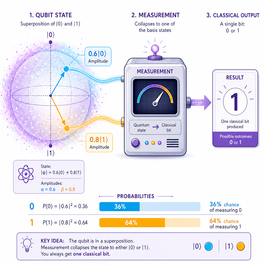
A qubit can be described by amplitudes before measurement, but when you measure it, you get one classical answer: 0 or 1.

For example, this state:

|ψ⟩ = 0.6|0⟩ + 0.8|1⟩

has probabilities:

P(0) = 0.6² = 0.36
P(1) = 0.8² = 0.64

After measurement, you don't observe both possibilities. You observe one outcome.

Important mental model

Quantum computing is not about “trying every answer and reading them all.” Measurement gives limited classical information. The power comes from designing gates so that wrong paths cancel out and useful paths become more likely.

Quantum gates are transformations

In classical programming, a function maps input values to output values:

f(input) -> output

A quantum gate transforms a state vector:

new_state = gate × old_state

One famous gate is the Hadamard gate, usually written H.

Applied to |0⟩, it creates an equal superposition:

H|0⟩ = (|0⟩ + |1⟩) / √2

Let's simulate that using plain Python matrix multiplication.

```python
import math

H = [
    [1 / math.sqrt(2),  1 / math.sqrt(2)],
    [1 / math.sqrt(2), -1 / math.sqrt(2)]
]

state_zero = [1.0, 0.0]

def apply_gate(gate, state):
    return [
        gate[0][0] * state[0] + gate[0][1] * state[1],
        gate[1][0] * state[0] + gate[1][1] * state[1]
    ]

def probabilities(state):
    return [abs(x) ** 2 for x in state]

new_state = apply_gate(H, state_zero)
probs = probabilities(new_state)

print("After applying H to |0>:")
print(f"state = [{new_state[0]:.3f}, {new_state[1]:.3f}]")
print(f"P(0) = {probs[0]:.2f}")
print(f"P(1) = {probs[1]:.2f}")
```

For a valid single-qubit state, the measurement probabilities must add up to ____.

Why amplitudes are not just probabilities

If qubits only stored probabilities, quantum computing would be much less interesting.

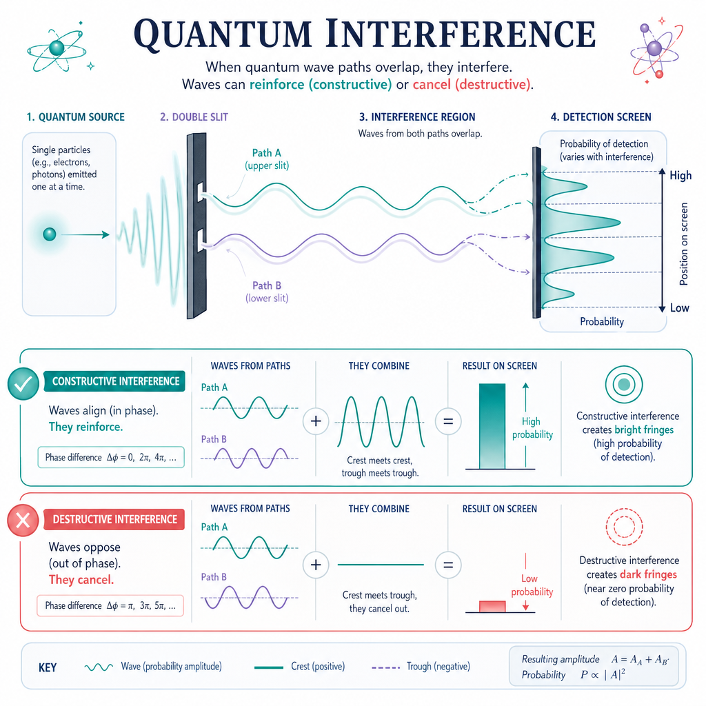
The special part is that amplitudes can be positive, negative, or complex. When gates combine amplitudes, they can interfere:

positive + positive -> larger amplitude
positive + negative -> cancellation

This is one of the central ideas behind quantum algorithms: arrange transformations so that bad answers cancel and useful answers become more likely.

You don't need the full algorithmic machinery yet. For now, remember:

Quantum programs manipulate amplitudes first, then measurement samples from the resulting probabilities.

Multiple qubits create larger state spaces

One qubit needs 2 amplitudes:

|0⟩, |1⟩

Two qubits need 4 amplitudes:

|00⟩, |01⟩, |10⟩, |11⟩

Three qubits need 8 amplitudes. In general:

n qubits -> 2ⁿ amplitudes

This exponential state space is part of why quantum systems are hard to simulate classically.

A famous two-qubit state is the Bell state:

(|00⟩ + |11⟩) / √2

It has a 50% chance of measuring 00, a 50% chance of measuring 11, and zero chance of 01 or 10.

```python
import math

# Two-qubit state vector order: |00>, |01>, |10>, |11>
bell_state = [
    1 / math.sqrt(2),
    0.0,
    0.0,
    1 / math.sqrt(2)
]

labels = ["00", "01", "10", "11"]

print("Bell state measurement probabilities:")
for label, amplitude in zip(labels, bell_state):
    probability = abs(amplitude) ** 2
    print(f"P({label}) = {probability:.2f}")
```

True or false: entanglement lets two computers send usable messages faster than light.

What to take forward

As a software developer, the first useful shift is not memorizing physics vocabulary. It's learning a new execution model.

Classical programming mindset:

state -> deterministic operations -> exact output

Quantum programming mindset:

amplitudes -> reversible transformations -> measurement probabilities

Practical implications

Quantum computers are not general replacements for classical systems. They are specialized tools that may help with certain problems in simulation, optimization, cryptography, and linear algebra.

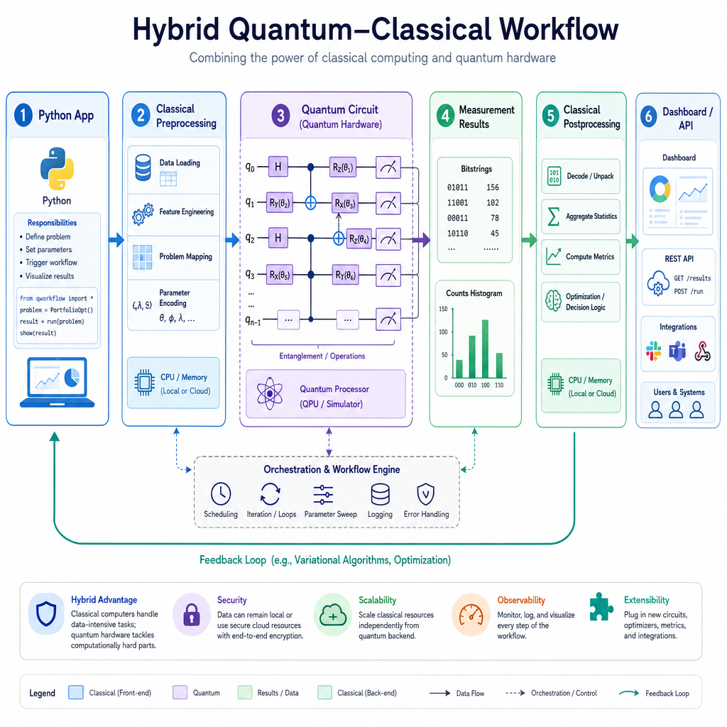
Your current Python and backend experience still matters: real quantum workflows need classical orchestration, data processing, APIs, experiment tracking, and visualization.

Next, we'll shift from quantum information to Introduction to Artificial Intelligence, where uncertainty appears again—but through models trained from data rather than qubit amplitudes.