Introduction to Neural Networks

Introduction

In this lesson, we will introduce the hot cake of the field of Machine Learning. Neural Networks are models designed based on our brains. Human brains have about 86 billion cells connected together by synapses. A neural network also has many cells/units that are connected to one another. Whenever an input is given, it is propagated through the entire network of cells, reaching the output cells where certain actions are handled for certain outputs.

This lesson will help you build a neural network from scratch. Later, we will introduce TensorFlow which is the de facto standard for neural networks. So let's get started.

How do human brains work?

Nerve cells are at the center of everything when it comes to brain functionality. A nerve cell neuron is a special biological cell that processes information. According to an estimation, there is a huge number of neurons, approximately $10^{11}$ with numerous interconnections. There are basically 4 parts of a neuron, then helps it to process and transfer information:

1. Synapses: Synapse is the connection point of two nerve cells.
2. Dendrites: They are tree-like branches, responsible for receiving the information from other neurons it is connected to. In another sense, we can say that they are like the ears of neurons.
3. Soma: It is the cell body of the neuron and is responsible for the processing of information, they have received from dendrites.
4. Axon: With this part, a cell transfers information to another cell (like wires).

Here is an image showing the connection of two neurons and their different parts.

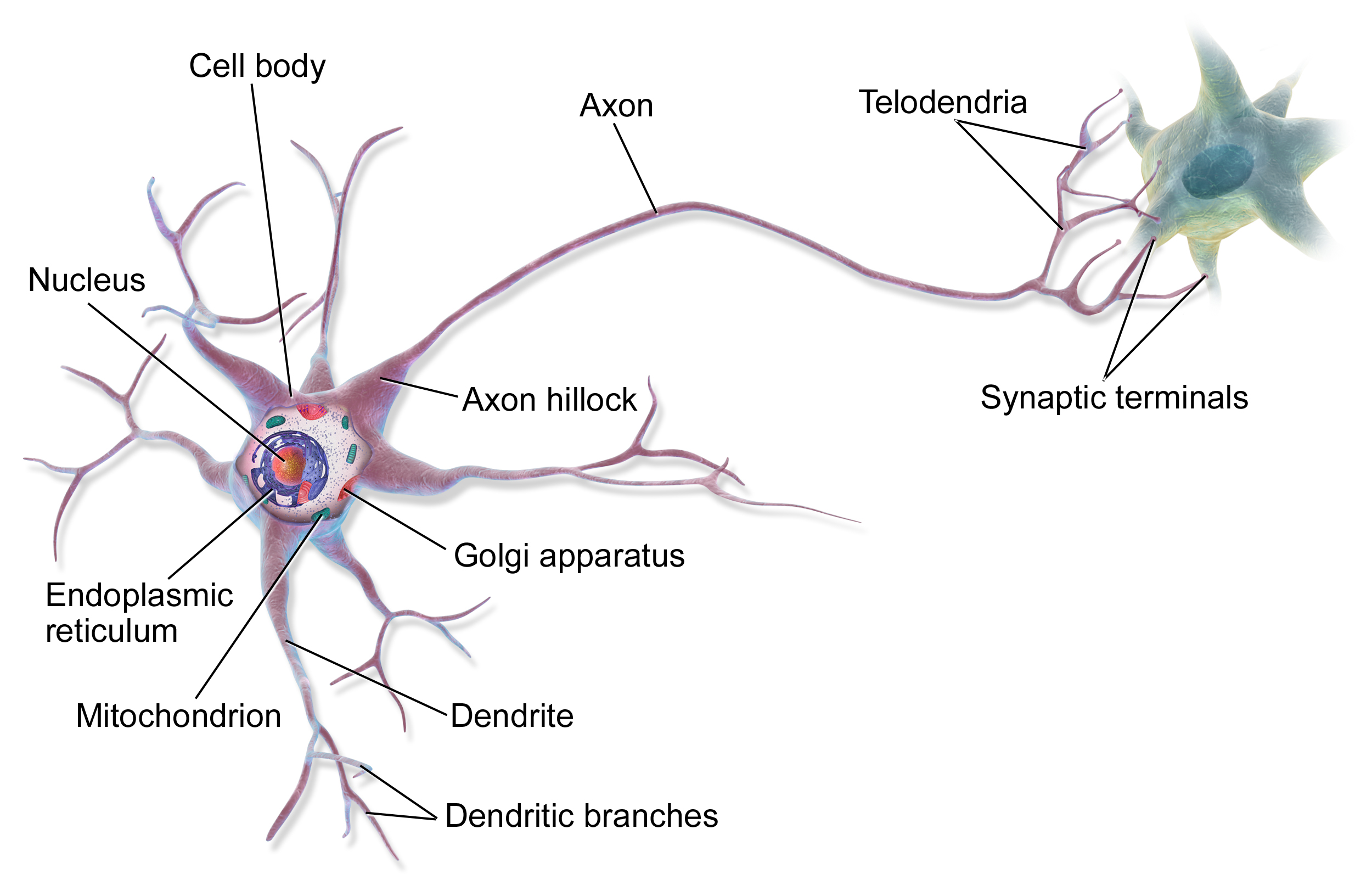
This is not a biology lesson, right? So why are we learning about brains? Because neural networks are nothing but brains created by humans. Below is the analogy in neural networks of what we have read about brains earlier:

1. Synapses are weights in an artificial neural network (ANN).
2. Dendrites are the input of a cell in ANN.
3. Soma is a node or unit cell in ANN.
4. Axon is the output of a cell in ANN.

Artificial Neuron

A neuron is a unit for computation in ANN. An ANN is nothing but a large network of neurons. There are different types of neurons, and there are many types of connections between neurons. All these varieties make different kinds of deep neural networks, some work well for tabular data, others work for images, and some work for sequential data like texts or speech.

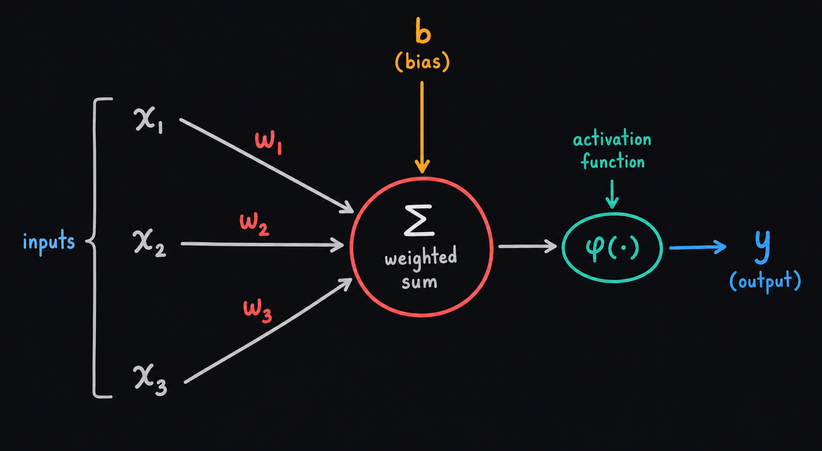
Here is the anatomy of a neuron in ANN.

Let us suppose the input has n features. So the input is like (X1, X2, X3... Xn). When this input data (more precisely a tensor) is given to the neural network, each of the features is multiplied by a weight. Then, all of them are summed up along with an additional bias value. This sum is the output of the neuron. Most of the time, to control this sum, an activation function is used. We will go through all of these in more detail.

$$a_1 = X_1 * W_1$$

$$a_2 = X_2 * W_2$$

$$a_3 = X_3 * W_3$$

$$...$$

$$a_n = X_n * W_n$$

The above can be written as:

$$a_i = X_i * W_i\ ;\ i \in {1, 2.. n}$$

Weighted Sum

Let us write the artificial neuron as a small equation. Each input feature is multiplied by its own weight, then all of those products are added together with a bias value.

$$z = x_1w_1 + x_2w_2 + ... + x_nw_n + b$$

After that, the activation function is applied:

$$output = activation(z)$$

The bias is important because it lets the neuron shift its decision even when the input values are small or zero. In simple words, weights control how much each feature matters, and bias controls where the neuron starts from.

```python
import numpy as np

X = np.array([0.2, 0.4, 0.6])
W = np.array([0.5, -0.3, 0.8])
b = 0.1

z = np.dot(X, W) + b
print(z)
```

Suppose X has shape (5, 3), where there are 5 samples and 3 features. A linear layer has 4 neurons. What should be the shape of the weight matrix W so that X @ W works?

Linear Layer

You might be thinking that we have to loop through all the features and then multiply them with the corresponding weights to get the output. But this will take forever for a very simple task. Remember, there could be thousands of features in an input (think of an image of size 4000*2000, then the number of pixels is 8000000). And this is only for one neuron. A modern ANN contains hundreds of such neurons.

The power of parallel processing with TPUs and GPUs has made this computation very fast and efficient. Graphics Processing Units (GPU) and Tensor Processing Units (TPU) can do matrix manipulation almost as fast as the CPU does simple arithmetics between two numbers. So we need to convert the above equations into matrix algebra.

Think of the input as a matrix where each column represents a feature and each row represents a sample.

Now we need to multiply all the features by the same weight for all samples. So we need to multiply each column by a value. If we consider a vector of weights of the same size as the number of features in input, then we can do matrix multiplication among them to get the desired result along with the summation.

But what about the BIAS we talked about??

The bias can also be added very easily in this matrix multiplication. That bias is appended to the weight vector in the first place. And a column (like a new feature) of 1 is appended in the first of the matrix $X$.

We have successfully understood the most basic part of deep learning, a layer of many unit cells. This is known as a linear layer. In deep learning, there will be a lot of layers joined together. Let's see how we can implement it in python.

class LinearLayer():
    # We will initialize W and b. They should be very small, so multiplying by 0.1
    def __init__(self, input_size, output_size, activation=None, name=None):
        self.W = np.random.randn(output_size, input_size) * 0.1
        self.b = np.random.randn(output_size, 1) * 0.1

        # Activation function are in the next section
        self.activation = activation
        if not activation:
            self.activation = IdentityActivation()

    # The is the prediction of the layer.
    def forward(X):
        self.A_prev = X.copy()
        self.Z_curr = np.dot(self.W, X) + self.b
        self.A_curr = self.activation.forward(self.Z_curr)
        return self.A_curr.copy()

## For our test purpose
if __name__ = '__main__':
    ll1 = LinearLayer(4, 1)
    print(ll1.forward([
        [1, 2, 3, 4]
    ])

Matrix multiplication is slower than for-loop multiplication because you also need to keep the order of the matrices.

Activation Function

As we said earlier, we also need activation functions to keep the output data in a diserable shape. There are a lot of activation functions used in deep learning. Let us discuss a few popular of them.

Identity Function

This is the simplest activation function. Sometimes you do not need to use any activation function for a specific layer. But to hold consistency across all layers, you need to create and store a dummy activation function for that layer. That activation function is the Identity function, which outputs whatever it is given as input.

$$f(x) = x$$

class IdentityActivation():
    def forward(X):
        return X

Linear

When the output value is proportional to the input value anywhere in the input domain, then the function is said to be a linear function. So, a linear function is just multiplying something with the input.

$$f(x) = a*x$$

class LinearActivation():
    def __init__(self, a):
        self.a = a

    def forward(X):
        return a*X

Sigmoid

Now the activation function will start to get interesting. The main objective of a sigmoid is to keep the output data between 0 and 1. The equation of this function is:

$$f(x) = \frac{1}{1+e^{-x}}$$

class SigmoidActivation():
    def forward(X):
        return 1/(1+np.e**(-X))

Tanh

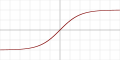
This activation function is very similar to sigmoid. The only difference is that the range of this function is [-1, 1]. And the equation used tanh function.

$$f(x) = tanh(x)$$

class TanhActivation():
    def forward(X):
        return np.tanh(X)

Binary Step

To make sure that the output is binary, a binary step activation function is used. This is mostly used when you are doing a binary classification. When the input is negative, the activation function outputs 0. And when it is positive, it outputs 1.

$$f(x) = 0\ if\ x \le 0\ ; 1\ otherwise$$

class BinaryStepActivation():
    def __init__(self, thresh=0):
        self.thresh = thresh

    def forward(X):
        out = np.ones_like(X)
        out[X <= 0] = 0
        return out

ReLU

Rectified Linear Unit Activation function has recently become popular for working very well with image datasets. It filters all the negative values to 0. For acts as a Linear Activation function for all the positive values.

$$f(x) = 0\ if\ x \le 0\ ;\ f_{linear}(x)\ otherwise$$

def ReLUActivation():
    def __init__(self, a):
        self.a = a
    def forward(X):
        out = X.copy()
        out[X <= 0] = 0
        out *= self.a

Leaky ReLU

Leaky ReLU is similar to ReLU, but it acts like another activation function instead of 0 when X is negative.

$$f(x) = b*x\ if\ x \le 0\ ;\ a*x(x)\ otherwise$$ $$b < a$$

class LeakyReLUActivation():
    def __init__(self,a,b):
        self.a = a
        self.b = b
    def forward(X):
        out = X.copy()
        out[X <= 0] *= self.b
        out[X > 0] *= self.a

SoftMax

SoftMax is a very different kind of activation function mostly used for multiclass classification. It takes all the outputs and then converts them to probability. The output of the softmax function will always add up to 1. And all the values of the output will be always non-negative.

$$f(x_i) = \frac{e^{x_i}}{\sum_{j=1}^J{e^{x_j}}}$$

As this is not a continuous function and depends on the individual value of x, it is quite difficult to plot on a 2D surface.

class SoftMaxActivation():
    def forward(X):
        return np.e**x / np.sum(np.e**x)

Which of the activation function's output is limited within 0 and 1?

Which of the activation function has a range between negative and positive infinity?

Neural Network with Feed Forward

So we have created linear layers and activation functions with forward methods. Our final class will be to create a NeuralNet which will contain everything it needs and provide an API to the user.

We will follow the Scikit-Learner API style for this. So there will be a predict method and a fit method (let's not worry about all other utility methods for now). As we have just implemented the forward methods for all the classes, let's create the predict method using those forward methods of all classes.

class NeuralNet():
    def __init__(self, layers=[]):
        self.layers = layers

    def predict(X):
        for layer in layers:
            A = layer.forward(A)
        return A

This looks easy, right? But now we will implement a little difficult part of the NeuralNet. The Backward Propagation.

Loss function

While training our neural network, we will need to calculate the loss depending on the prediction of the network, and target labels. We can simply use a function to implement the loss function equation of categorical cross-entropy.

def categorical_crossentropy(target, output):
    output /= output.sum(axis=-1, keepdims=True)
    output = np.clip(output, 1e-7, 1 - 1e-7) # So that weights dont become 0
    return np.sum(target * -np.log(output), axis=-1, keepdims=False)

Backward Propagation

We have already learned about the gradient descent algorithm in lesson 4. We will discuss the same and apply it to the neural networks backpropagation method. We already have the NeuralNet class along with other layers. All we need to do is add a new method called backward to each of them so that it is possible to do backward propagation to the network.

What will the backward method do in each case? The backward method will output the gradient of the input, with respect to W. The input we just mentioned is not X, it is the gradient we got from another layer.

Remember, gradient descendent algorithm and backward propagation are different algorithms. The first one is used only to get the gradient of the loss with respect to W. The second one is responsible for updating the weights using that gradient taken from the first algorithm.

You will understand this better if you take a look at the following equations. Nerd Alert! Calculus Ahead.

$$dW^{[l]} = \frac{\partial L}{\partial W^{[l]}} = \frac{1}{m} dZ^{[l]} A^{[l-1] T}$$

$$db^{[l]} = \frac{\partial L}{\partial b^{[l]}} = \frac{1}{m} dZ^{l} $$

$$dA^{[l-1]} = \frac{\partial L}{\partial A^{[l-1]}} = W^{[l] T} dZ^{[l]}$$

$$dZ^{[l]} = dA^{[l]} * g'(Z[l])$$

After calculating gradients of all the layers and activation functions using the above equations, we can update the weights via:

$$W^{[l]} = W^{[l]} - \alpha dW^{[l]}$$

$$b^{[l]} = b^{[l]} - \alpha db^{[l]}$$

Let us implement this in python. We are only implementing it on the LinearLayer class, sigmoid, and relu activation functions. You can look at the derivative of other activation functions here.

class SigmoidActivation():
    # ...
    def backward(self, A):
        # Just the derivative
        return A*(1-A)

class ReLUActivation():
    # ...
    def backward(self, A):
        A = A.copy()
        A[A <= 0] = 0;
        A *= self.a
        return A;

class LinearLayer():
    # ...
    def backward(dA_curr, lr=0.001):
        m = A_prev.shape[1]

        dZ_curr = self.activation.backward(dA_curr, self.Z_curr)
        dW_curr = np.dot(dZ_curr, self.A_prev.T) / m
        db_curr = np.sum(dZ_curr, axis=1, keepdims=True) / m
        dA_prev = np.dot(self.W.T, dZ_curr)

        self.W -= lr * dW_curr
        self.b -= lr * db_curr

        return dA_prev

Now that we have the method backward for all classes, we can implement the fit method in our NeuralNet class.

class NeuralNet():
    # ...
    def fit(X, y, lr=0.001, epoch=1):
        for i in range(epoch):
            for layer in self.layers:
                X = layer.forward(X)

            dA_curr = categorical_crossentropy(y, X)

            for layer in reversed(self.layers):
                dA_curr, = layer.backward(dA_curr, lr=self.lr)

Now the only work left is to instantiate and train the model. We will train it on the iris dataset we discussed in the Scikit-learn chapter.

from sklearn.datasets import load_iris
from sklearn.metrics import accuracy_score # To calculate accuracy

iris = load_iris()

net = NeuralNet([
    LinearLayer(4, 10, activation=ReLUActivation()),
    LinearLayer(10, 5, activation=ReLUActivation()),
    LinearLayer(5, 3, activation=SoftMaxActivation()),
])

# We do preprocessing like the last lesson
X_train, X_test, y_train, y_test = train_test_split(iris.data, iris.target, test_size=0.25, random_state=42)

net.fit(X_train, y_train)
pred = net.predict(X_test)
print(accuracy_score(pred, y_test))

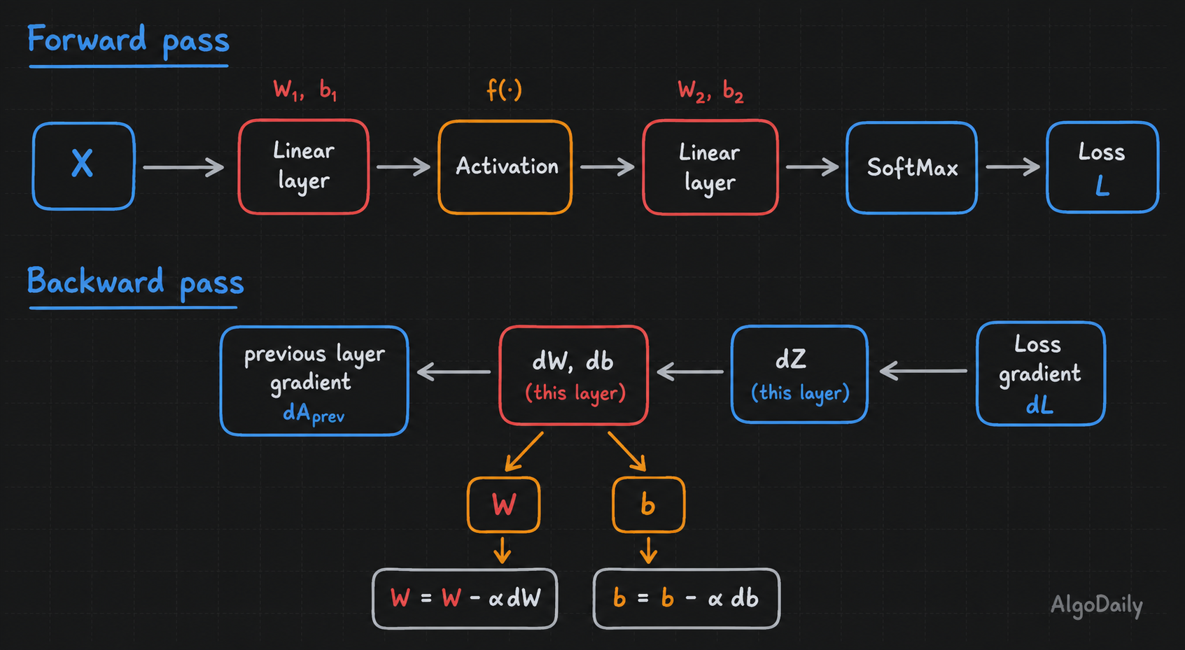
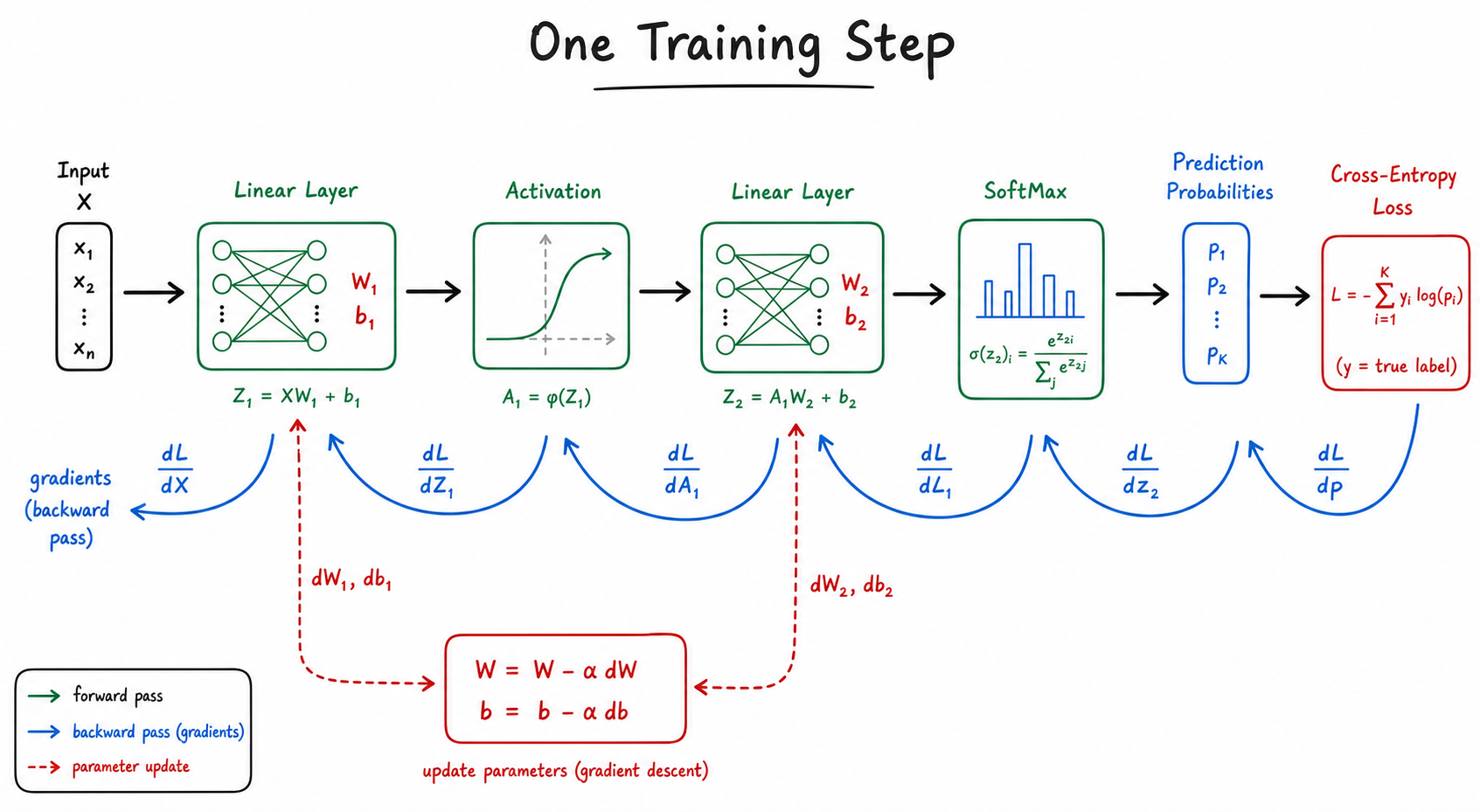
Before the training loop, lock in the direction of information flow:

• Forward pass: inputs become predictions, then loss.
• Backward pass: loss sends gradients backward through each layer.
• Update step: weights and biases move a small amount using those gradients.

The key interview idea: backpropagation computes dW and db; gradient descent uses them to update W and b.

Before moving on, connect the pieces: a neural network does not just predict once. Training repeats a loop.

Notice the direction change: feed forward turns inputs into probabilities and loss; backpropagation moves gradients backward through the same layers; the update step nudges weights and biases to reduce future loss.

Conclusion

Congratulations. You can successfully create a full-fledged Neural Network architecture. The network has many activation functions, can input 2-dimensional data with any shape, and can be as deep or as wide as you need.

I understand that all of the code and the mathematical backgrounds are tough for you. In real life, you do not have to do any of these at all. In the next lesson, we will learn TensorFlow. Then you will realize how easy it is to create and train a deep learning model within as small as 10 lines of code.

One Pager Cheat Sheet

• Neural Networks are models, designed based on our brains, that propagate inputs through many cells/units to handle certain outputs when given an input.
• Nerve cells process and transfer information through Synapses, Dendrites, Soma and Axon to work, which is effectively simulated in Artificial Neural Networks (ANNs) to mimic the operation of a human brain.
• A neuron in an Artificial Neural Network (ANN) computes an output (activation) by multiplying the inputs (tensor) with weights and adding a bias, and then often applying an activation function to the sum.
• A Linear Layer is an efficient way of implementing a single neuron using matrix multiplication, which makes it possible to do parallel processing with GPUs and TPUs.
• Matrix multiplication is more efficient than for-loops due to its ability to take advantage of parallel processing and be performed in any random order.
• An activation function is used to keep the output data in a desired shape in deep learning.
• The IdentityActivation function returns the given input X as its output.
• A linear function is multiplied by an input X and produces an output which is proportional to the input for all values of the input domain, which can be seen in the equation f(x) = a*x.
• The Sigmoid activation function takes in a value and produces a output between 0 and 1 to classify the data, represented by the equation f(x) = 1/(1+e^-x).
• The Tanh activation function ranges from -1 to 1 and is calculated using the tanh() function.
• The activation function Binary Step is a threshold-based activation used for binary classification, which outputs 0 if the input is negative, and 1 if it is positive.
• TheReLUActivation function filters negative values to 0 and acts as a linear function with all the positive values.
• Leaky ReLU is a type of activation function defined by the equation f(x) = b*x when x <= 0 and a*x when x > 0, with b < a, which can be implemented in Python through the LeakyReLUActivation class.
• The SoftMax activation function is a complex non-continuous function which helps convert outputs to probabilities and is mostly used for multiclass classification, demonstrated by the Python code snippet provided.
• The sigmoid activation function provides outputs between 0 and 1, while SoftMax converts all outputs to a total probability of 1.
• The Leaky ReLU activation function is defined by f(x) = ax when x<0 and f(x) = x when x>=0, with a range of negative to positive infinity, which is in contrast to other activation functions such as the Sigmoid.
• We have created a NeuralNet class which provides an API for the user to predict using the forward methods of other classes.
• We can calculate the loss of our neural network with the categorical_crossentropy function, which performs the Categorical Cross-Entropy equation.
• We can implement backpropagation in neural networks by adding a backward() method that outputs the gradient of the input with respect to W and by using gradient descent algorithm in combination with backward propagation to update the weights and biases.
• - Backprop computes gradients layer by layer; gradient descent applies the parameter update.
• - Neural network training cycles through forward pass → loss → backward gradients → weight update.
• With a few lines of code in TensorFlow, you can easily create and train a deep learning model to input 2-dimensional data of any shape.