Predictive Modeling and Strategy Automation in R
Read at your own pace. Code execution, quizzes, progress tracking, and the AI tutor are available in the interactive view with JavaScript enabled.
Automation Finish Line
Why this lesson matters
You now have the full input side of a dynamic trading system:
- In Accessing and Streaming OHLC Data from APIs and Web-Sockets in R, you built the ingestion mindset.
- In Resampling and Aggregating Time-Frame Data in R, you turned second-level events into aligned 30-minute and 60-minute bars.
- In Building a Real-Time Algorithmic Trading Framework in R, you created a stateful loop that emits one feature row at a time.
Now we finish the pipeline: use those feature rows to train a simple predictive model, generate live predictions, and convert predictions into automated strategy decisions.
The examples below use executable Python syntax, but the structure maps directly to the same data-frame workflow you would implement in R with
data.table,xts, ortidyverse.

Modeling Target
Predict the next thing, not the current thing
A predictive model needs two pieces:
-
Features: information available now, such as:
- current close
- distance from 30-minute 21-period moving average
- distance from 60-minute 21-period moving average
- spread between those two moving averages
-
Target: what you want to predict later, such as:
- next-bar return
- next-bar direction
- future volatility
- probability of crossing a moving average
For a first dynamic strategy, use a simple target:
target = next_close - current_close
That keeps the lesson focused on the live system mechanics rather than advanced ML.
```python
import numpy as np
import pandas as pd

np.random.seed(7)

# Simulated feature rows, as if emitted by the framework from the previous lesson.
# In production, ma30_21 and ma60_21 would come from your aligned timeframe engine.
n = 160
ts = pd.date_range("2024-01-01 09:30", periods=n, freq="min")
close = 100 + np.cumsum(np.random.normal(0, 0.12, n))

# Demo approximations of already-built multi-timeframe features.
ma30_21 = pd.Series(close).rolling(30, min_periods=30).mean()
ma60_21 = pd.Series(close).rolling(60, min_periods=60).mean()

features = pd.DataFrame({
    "ts": ts,
    "close": close,
    "ma30_21": ma30_21,
    "ma60_21": ma60_21
}).dropna().reset_index(drop=True)

features["dist_30"] = features["close"] - features["ma30_21"]
features["dist_60"] = features["close"] - features["ma60_21"]
features["ma_spread"] = features["ma30_21"] - features["ma60_21"]
features["target_next_change"] = features["close"].shift(-1) - features["close"]

train = features.dropna().copy()
X = train[["dist_30", "dist_60", "ma_spread"]].to_numpy()
y = train["target_next_change"].to_numpy()

# Add intercept column and fit linear regression with least squares.
X_design = np.column_stack([np.ones(len(X)), X])
beta = np.linalg.lstsq(X_design, y, rcond=None)[0]

latest = features.iloc[-1]
latest_x = np.array([1, latest["dist_30"], latest["dist_60"], latest["ma_spread"]])
predicted_next_change = float(latest_x @ beta)

print("Rows used for training:", len(train))
print("Coefficients:", np.round(beta, 6).tolist())
print("Latest timestamp:", latest["ts"])
print("Latest close:", round(latest["close"], 4))
print("Predicted next close change:", round(predicted_next_change, 6))
```
Avoiding Leakage
You are training a model that predicts the next bar's price change. Which feature setup is safest for live trading?
Model As Function
Keep the model boring on purpose
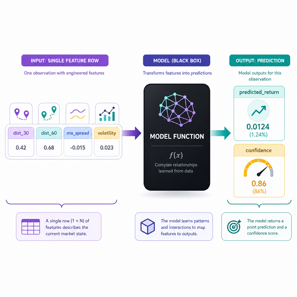
In a real-time trading loop, your model should behave like a plain function:
feature_row -> prediction
That means the live engine does not need to know the math details of linear regression. It only needs to know:
- what columns the model expects
- whether the model is trained
- how to call
predict - how to handle missing or stale features
This separation is powerful. You can start with linear regression, then later swap in ridge regression, random forests, gradient boosting, or another model without rewriting the ingestion and timeframe code.
Live Prediction Loop
Add prediction to the stateful framework
From the previous lesson, you already have the mental model:
new event -> update state -> emit feature row
Now extend it:
new event -> update state -> emit feature row -> predict -> decide
In production, your feature row would include aligned 30-minute and 60-minute 21-period moving averages. To keep this example compact and executable, the code uses shorter rolling windows while preserving the same dynamic structure.
```python
import numpy as np
import pandas as pd

np.random.seed(11)

class LinearModel:
    def __init__(self):
        self.beta = None
        self.columns = ["dist_fast", "dist_slow", "ma_spread"]

    def fit(self, df):
        train = df.dropna().copy()
        if len(train) < 15:
            return False
        X = train[self.columns].to_numpy()
        y = train["target_next_change"].to_numpy()
        X_design = np.column_stack([np.ones(len(X)), X])
        self.beta = np.linalg.lstsq(X_design, y, rcond=None)[0]
        return True

    def predict_one(self, row):
        if self.beta is None:
            return None
        x = np.array([1] + [row[c] for c in self.columns])
        return float(x @ self.beta)


def decide(pred, threshold=0.025):
    if pred is None:
        return "WAIT"
    if pred > threshold:
        return "BUY"
    if pred < -threshold:
        return "SELL"
    return "HOLD"

closes = []
feature_rows = []
model = LinearModel()

price = 100.0
for i in range(75):
    ts = pd.Timestamp("2024-01-01 09:30") + pd.Timedelta(minutes=i)
    price += np.random.normal(0, 0.10)
    closes.append(price)

    if len(closes) < 12:
        continue

    fast_ma = np.mean(closes[-5:])
    slow_ma = np.mean(closes[-12:])

    row = {
        "ts": ts,
        "close": price,
        "dist_fast": price - fast_ma,
        "dist_slow": price - slow_ma,
        "ma_spread": fast_ma - slow_ma
    }
    feature_rows.append(row)

    df = pd.DataFrame(feature_rows)
    df["target_next_change"] = df["close"].shift(-1) - df["close"]

    # Retrain periodically. In real systems, this might be scheduled or triggered.
    if i % 10 == 0:
        trained = model.fit(df)
        if trained:
            print(f"{ts} | retrained on {df.dropna().shape[0]} rows")

    pred = model.predict_one(row)
    action = decide(pred)

    if i >= 68:
        printable_pred = None if pred is None else round(pred, 5)
        print(f"{ts} | close={price:.3f} | pred={printable_pred} | action={action}")
```
Closed Bars Only
True or false: for a live strategy, it is usually safer to generate model features from completed bars than from bars that are still forming.
Prediction To Action
A prediction is not an order
This is one of the most important distinctions in automated trading.
A model says:
I expect the next change to be +0.04
A strategy policy decides:
Is that large enough?
Am I already in a position?
What is my max risk?
Is the market open?
Is the data fresh?
Should I send an order?
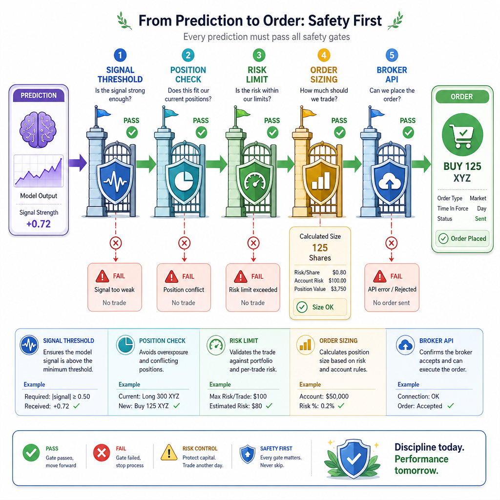
A practical live decision stack looks like this:
prediction
  -> signal threshold
  -> position rules
  -> risk limits
  -> order sizing
  -> broker/API command
Do not let the ML model directly place orders. Put a risk and policy layer between prediction and execution.
Policy Layer
Fill in the blank:
In a robust automated trading system, the model should produce a prediction, but a separate ______ layer should decide whether that prediction is allowed to become an order.
Backtest Live Parity
Use the same decision function twice
A common beginner mistake is writing one strategy for backtesting and another for live trading.
Instead, keep the core decision logic reusable:
prediction + current_position + risk_config -> action
Then call the same function from:
- historical simulation
- paper trading
- live trading
This makes your backtest more honest because the live system is using the same rules.
```python

def strategy_decision(prediction, position, threshold=0.03, max_position=1):
    """Return one of: BUY, SELL, EXIT, HOLD."""
    if prediction is None:
        return "HOLD"

    if prediction > threshold and position < max_position:
        return "BUY"
    if prediction < -threshold and position > -max_position:
        return "SELL"
    if abs(prediction) < threshold / 2 and position != 0:
        return "EXIT"
    return "HOLD"

# Historical predictions from a backtest run.
backtest_predictions = [0.01, 0.05, 0.02, -0.04, -0.01, 0.00]

# Same values arriving one by one in a simulated live loop.
live_predictions = list(backtest_predictions)

position = 0
backtest_actions = []
for pred in backtest_predictions:
    action = strategy_decision(pred, position)
    backtest_actions.append(action)
    if action == "BUY":
        position += 1
    elif action == "SELL":
        position -= 1
    elif action == "EXIT":
        position = 0

position = 0
live_actions = []
for pred in live_predictions:
    action = strategy_decision(pred, position)
    live_actions.append(action)
    if action == "BUY":
        position += 1
    elif action == "SELL":
        position -= 1
    elif action == "EXIT":
        position = 0

print("Backtest actions:", backtest_actions)
print("Live actions:    ", live_actions)
print("Same logic used:", backtest_actions == live_actions)
```
Course Blueprint
The complete dynamic trading loop
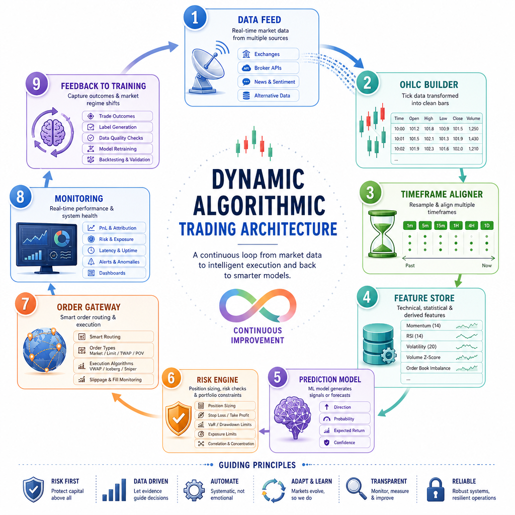
You now have the end-to-end blueprint:
1. Ingest second-level data
2. Validate and normalize events
3. Build OHLC bars
4. Resample into 30-minute and 60-minute frames
5. Align timeframe features into one row
6. Update strategy state
7. Predict with a model
8. Apply risk and decision rules
9. Send, log, or simulate orders
10. Monitor drift, errors, and performance
The key idea is that every live event should move through the same pipeline shape. The model is only one component.
For your next real project, keep it simple:
- start with paper trading
- log every feature row and prediction
- compare live decisions to backtest decisions
- retrain on a schedule, not randomly
- never place orders without freshness checks and risk limits
You have gone from raw OHLC ingestion to a usable real-time predictive strategy architecture.