Risk Management in C++

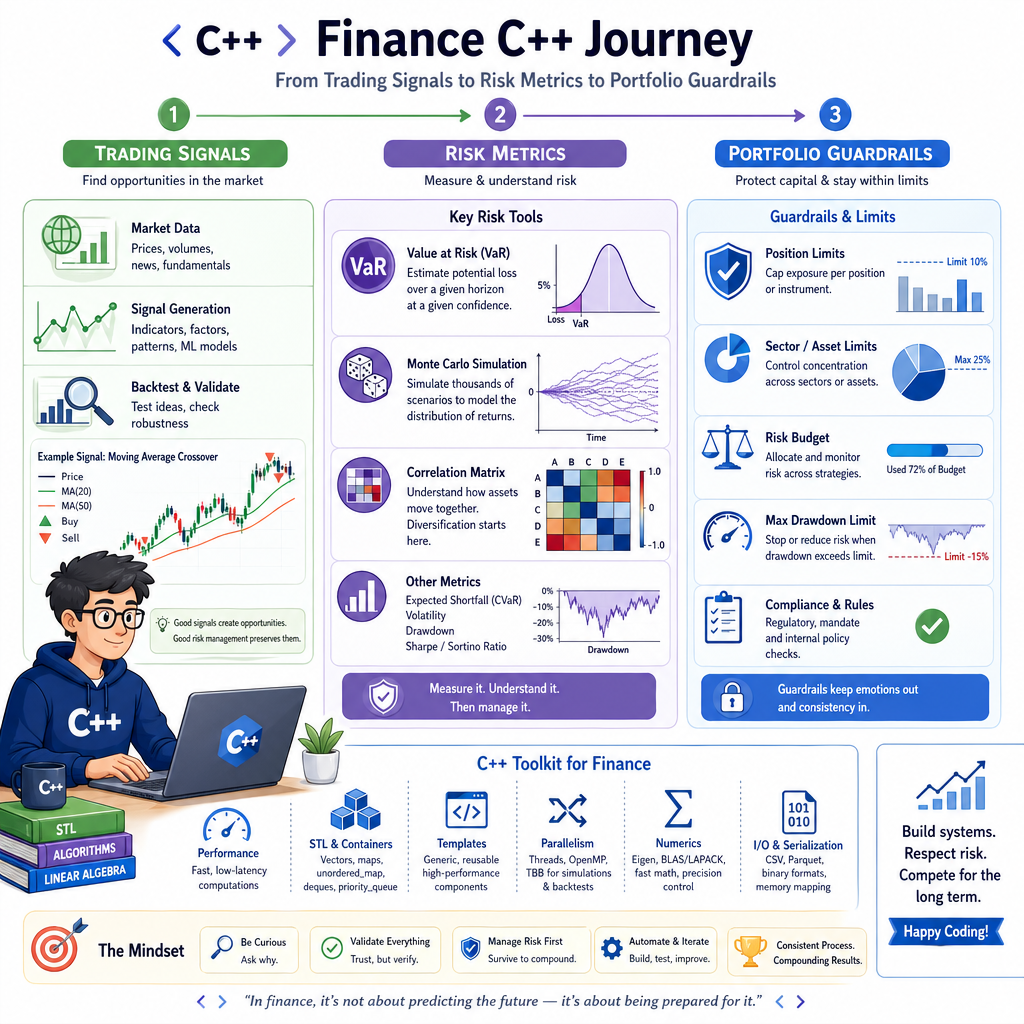
From trading to surviving

In Algorithmic Trading with C++, you built the basic loop: market data -> signal -> backtest -> execution boundary.

Risk management asks the next desk-level question:

If this strategy is wrong, how bad can it get?

In finance, returns matter, but survival matters more. A strategy that makes money most days but can blow up on one bad day is like maxing out every basketball possession with no defense or recovery plan.

Today we will use C++ to model:

• VaR: a downside loss threshold
• Monte Carlo simulation: many possible futures
• Risk modeling: volatility, correlation, and loss distributions
• Portfolio optimization: choosing weights with risk in mind

We will keep this scoped to risk engines. In the next lesson, Financial Data Analysis with C++, you will go deeper on analyzing larger datasets.

The basic risk engine

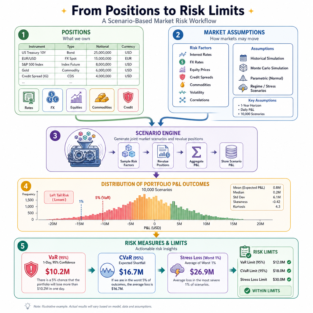
A risk engine usually transforms positions and market assumptions into a distribution of possible losses.

Positions + Market Assumptions
          |
          v
     Scenario Engine
          |
          v
   Portfolio P&L Outcomes
          |
          v
 Risk Metrics: VaR, CVaR, limits

Think of this like training volume in bodybuilding: one workout is not the whole story. You care about the distribution of outcomes over time: normal sessions, hard sessions, injury risk, and recovery.

In C++, this maps naturally to data structures you have already seen:

• std::vector<double> for prices, returns, losses, weights
• functions for reusable calculations
• sorting for percentile-based metrics
• random number generation for simulations

We are not replacing financial judgment with code. We are making the assumptions visible and testable.

A portfolio has a 1-day 95% VaR of $50,000.

What is the best interpretation?

VaR from historical returns

The simplest VaR approach uses past returns as possible future scenarios.

Steps:

1. Convert prices into returns.
2. Convert returns into portfolio profit/loss.
3. Convert P&L into losses.
4. Sort losses.
5. Pick a high percentile, such as 95%.

This is not a perfect forecast. It says: if tomorrow looked like one of these historical days, how bad is the tail?

Here is a small standalone C++ example.

```cpp
#include <algorithm>
#include <cmath>
#include <iomanip>
#include <iostream>
#include <vector>

int main() {
    std::vector<double> prices = {100.0, 101.5, 99.0, 98.0, 102.0, 97.5, 96.0, 99.5, 101.0, 95.0, 97.0};

    double shares = 1000.0;
    double currentPrice = prices.back();
    double portfolioValue = shares * currentPrice;

    std::vector<double> losses;

    for (std::size_t i = 1; i < prices.size(); ++i) {
        double dailyReturn = (prices[i] - prices[i - 1]) / prices[i - 1];
        double pnl = portfolioValue * dailyReturn;
        double loss = -pnl;
        losses.push_back(loss);
    }

    std::sort(losses.begin(), losses.end());

    double confidence = 0.95;
    std::size_t index = static_cast<std::size_t>(std::ceil(confidence * losses.size())) - 1;
    double var95 = losses[index];

    std::cout << std::fixed << std::setprecision(2);
    std::cout << "Portfolio value: $" << portfolioValue << "\n";
    std::cout << "Historical 95% VaR: $" << var95 << "\n";

    std::cout << "Sorted losses: ";
    for (double loss : losses) {
        std::cout << "$" << loss << " ";
    }
    std::cout << "\n";

    return 0;
}
```

True or false?

If a portfolio has a 99% VaR of $1 million, then the portfolio cannot lose more than $1 million in one day.

Simulating many futures

Historical VaR only reuses past days. Monte Carlo simulation creates many possible future returns from a model.

For a basic one-asset example, we assume:

• annual expected return mu
• annual volatility vol
• one trading day, roughly 1 / 252 of a year
• normally distributed random shocks

This is a model, not reality. The value is that you can quickly generate thousands of possible outcomes and inspect the tail.

In production, model choice matters a lot. But the C++ mechanics are already useful: random engines, vectors, sorting, and percentiles.

```cpp
#include <algorithm>
#include <cmath>
#include <iomanip>
#include <iostream>
#include <random>
#include <vector>

int main() {
    const int simulations = 50000;
    const double portfolioValue = 1'000'000.0;
    const double mu = 0.08;       // annual expected return
    const double vol = 0.22;      // annual volatility
    const double dt = 1.0 / 252.0;
    const double confidence = 0.99;

    std::mt19937 rng(42);
    std::normal_distribution<double> normal(0.0, 1.0);

    std::vector<double> losses;
    losses.reserve(simulations);

    for (int i = 0; i < simulations; ++i) {
        double z = normal(rng);
        double logReturn = (mu - 0.5 * vol * vol) * dt + vol * std::sqrt(dt) * z;
        double endingValue = portfolioValue * std::exp(logReturn);
        double loss = portfolioValue - endingValue;
        losses.push_back(loss);
    }

    std::sort(losses.begin(), losses.end());

    std::size_t varIndex = static_cast<std::size_t>(std::ceil(confidence * losses.size())) - 1;
    double var99 = losses[varIndex];

    double tailSum = 0.0;
    int tailCount = 0;
    for (std::size_t i = varIndex; i < losses.size(); ++i) {
        tailSum += losses[i];
        ++tailCount;
    }
    double cvar99 = tailSum / tailCount;

    std::cout << std::fixed << std::setprecision(2);
    std::cout << "Monte Carlo 1-day 99% VaR: $" << var99 << "\n";
    std::cout << "Monte Carlo 1-day 99% CVaR: $" << cvar99 << "\n";
    std::cout << "Worst simulated loss: $" << losses.back() << "\n";

    return 0;
}
```

Fill in the blank:

A method that estimates risk by generating many random possible market outcomes is called ______ simulation.

Risk is not just asset-by-asset

A portfolio can be less risky than its parts if the assets do not move together.

For two assets, portfolio variance is:

variance = wA^2 * varA
         + wB^2 * varB
         + 2 * wA * wB * covarianceAB

Where:

• wA, wB are portfolio weights
• varA, varB are individual variances
• covarianceAB = correlation * volA * volB

This is where correlation matters. Two players both scoring 30 is great, but if both only perform in the same exact matchup, your team is more fragile. Diversification comes from different behavior under different conditions.

The code below scans possible weights and finds the lowest-volatility mix for two assets.

```cpp
#include <cmath>
#include <iomanip>
#include <iostream>

int main() {
    double volA = 0.18;   // annual volatility of asset A
    double volB = 0.30;   // annual volatility of asset B
    double rho = 0.25;    // correlation between assets

    double varA = volA * volA;
    double varB = volB * volB;
    double covariance = rho * volA * volB;

    double bestWeightA = 0.0;
    double bestVol = 1e9;

    for (int i = 0; i <= 100; ++i) {
        double wA = i / 100.0;
        double wB = 1.0 - wA;

        double portfolioVariance =
            wA * wA * varA +
            wB * wB * varB +
            2.0 * wA * wB * covariance;

        double portfolioVol = std::sqrt(portfolioVariance);

        if (portfolioVol < bestVol) {
            bestVol = portfolioVol;
            bestWeightA = wA;
        }
    }

    std::cout << std::fixed << std::setprecision(2);
    std::cout << "Minimum-volatility allocation:\n";
    std::cout << "Asset A weight: " << bestWeightA * 100.0 << "%\n";
    std::cout << "Asset B weight: " << (1.0 - bestWeightA) * 100.0 << "%\n";
    std::cout << "Annualized portfolio volatility: " << bestVol * 100.0 << "%\n";

    return 0;
}
```

Metrics become guardrails

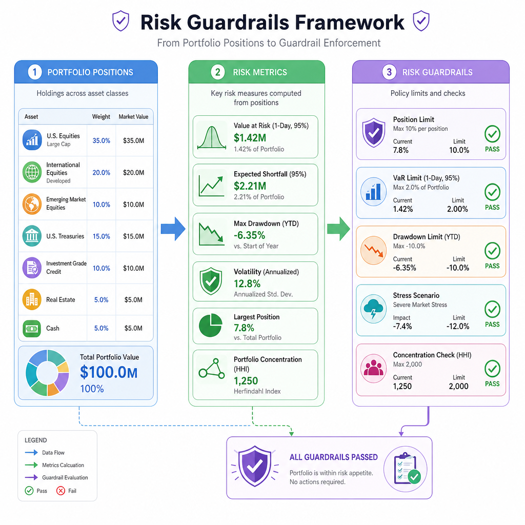
A risk number is useful only if it changes behavior.

Common controls include:

• Position limits: do not let one trade dominate the book
• VaR limits: reduce exposure if modeled tail loss is too high
• Drawdown limits: stop trading or resize after cumulative losses
• Stress scenarios: test specific shocks, such as rates jumping or equities dropping
• Concentration checks: avoid hidden dependence on one sector, asset, or factor

A good C++ risk module should be boring in the best way:

input positions -> compute risk -> compare limits -> report action

For someone coming from JavaScript, this is similar to backend validation. The difference is that the validation protects capital, not just form data.

A strategy has strong average returns, but one asset now represents 70% of total exposure.

Which risk control is most directly relevant?

What you can now build

You have moved from writing trading logic to asking risk-desk questions:

• What is the modeled downside loss?
• What happens in the tail?
• How do many simulated futures change the picture?
• How do portfolio weights and correlations affect volatility?
• When should a system reduce or block exposure?

The big C++ lesson is that risk management is mostly data transformation plus disciplined assumptions:

prices/positions -> returns/scenarios -> P&L -> losses -> limits

That pattern will keep showing up in finance codebases. Next, you will shift toward Financial Data Analysis with C++, where the focus becomes cleaning, summarizing, and extracting insight from financial datasets.