Understanding Big O Notation and Algorithmic Complexity

Read at your own pace. Code execution, quizzes, progress tracking, and the AI tutor are available in the interactive view with JavaScript enabled.

Introduction

Algorithm Complexity and Big O Notation

**Objective**: In this lesson, we'll cover the topics of `Algorithm Complexity and Big O Notation`. By the end, you should: - Be familiar with these terms and what they mean. - See their use in practice. - Use these tools to measure how "good" an algorithm is.

In software engineering, developers can write a program in several ways.

For instance, there are many ways to search an item within a data structure. You can use linear search, binary search, jump search, interpolation search, among many other options.

Our focus in this lesson is on mastering Algorithm Complexity and Big O Notation. But what we want to do with this knowledge is to improve the performance of a software application. This is why it's important to understand which algorithm to use, depending upon the problem at hand.

Let's start with basics. A computer algorithm is a series of steps the machine takes in order to take an input and compute an output. There are several ways to measure its performance. One of the metrics used to compare algorithms is using this notion of algorithm complexity.

Sounds challenging, doesn't it? Don't worry, we'll break it down.

Algorithm complexity can be further divided into two types: time complexity and space complexity. Let's briefly touch on these two:

The time complexity, as the name suggests, refers to the time taken by the algorithm to complete its execution.
The space complexity refers to the memory occupied by the algorithm.

In this lesson, we will study time and space complexity with the help of many examples. Before we jump in, let’s see an example of why it is important to measure algorithm complexity.

Importance Of Algorithm Complexity

Importance of Algorithm Complexity

To study the importance of algorithm complexity, let’s write two simple programs. Both the programs raise a number x to the power y.

Here's the first program: see the sample code for Program 1.

```python
def custom_power(x, y):
    result = 1
    for i in range(y):
        result = result * x
    return result

print(custom_power(3, 4))
```
```js
function customPower(x, y) {
    let result = 1;
    for (let i = 0; i < y; i++) {
        result = result * x;
    }
    return result;
}


console.log(customPower(3, 4));
```
```java
public class Main {
    public static long customPower(int x, int y) {
        long result = 1;
        for (int i = 0; i < y; i++) {
            result = result * x;
        }
        return result;
    }

    public static void main(String[] args) {
        System.out.println(customPower(3, 4));
    }
}
```
```cpp
#include <iostream>

long customPower(int x, int y) {
    long result = 1;
    for (int i = 0; i < y; i++) {
        result = result * x;
    }
    return result;
}

int main() {
    std::cout << customPower(3, 4) << std::endl;
    return 0;
}
```
```csharp
using System;

class Program {
    public static long CustomPower(int x, int y) {
        long result = 1;
        for (int i = 0; i < y; i++) {
            result = result * x;
        }
        return result;
    }

    static void Main(string[] args) {
        Console.WriteLine(CustomPower(3, 4));
    }
}
```
```go
package main

import "fmt"

func customPower(x, y int) int {
    result := 1
    for i := 0; i < y; i++ {
        result = result * x;
    }
    return result
}

func main() {
    fmt.Println(customPower(3, 4))
}
```

Step Three

Let’s now see how much time the previous function takes to execute. In a Jupyter Notebook or any language interpreter, you can use the following script to find the time taken by the algorithm.

```python
from timeit import timeit

func = '''
def custom_power(x, y):
    result = 1
    for i in range(y):
        result = result * x
    return result
'''

t = timeit("custom_power(3,4)", setup=func)
print(t)
```
```js
function customPower(x, y) {
    let result = 1;
    for (let i = 0; i < y; i++) {
        result = result * x;
    }
    return result;
}


var start = new Date().getTime();
console.log(customPower(3, 4));
var end = new Date().getTime();

console.log(`Call to customPower took ${end - start} milliseconds`);
```
```java
public class Main {
    public static long customPower(int x, int y) {
        long result = 1;
        for (int i = 0; i < y; i++) {
            result = result * x;
        }
        return result;
    }

    public static void main(String[] args) {
        long startTime = System.nanoTime();
        System.out.println(customPower(3, 4));
        long endTime = System.nanoTime();

        long duration = endTime - startTime;
        System.out.println(duration + " nanoseconds");
    }
}
```
```cpp
#include <iostream>
#include <chrono>

long customPower(int x, int y) {
    long result = 1;
    for (int i = 0; i < y; i++) {
        result = result * x;
    }
    return result;
}

int main() {
    auto start = std::chrono::high_resolution_clock::now();
    std::cout << customPower(3, 4) << std::endl;
    auto end = std::chrono::high_resolution_clock::now();

    auto duration = std::chrono::duration_cast<std::chrono::nanoseconds>(end - start);
    std::cout << duration.count() << " nanoseconds" << std::endl;
    return 0;
}
```
```csharp
using System;
using System.Diagnostics;

class Program {
    public static long CustomPower(int x, int y) {
        long result = 1;
        for (int i = 0; i < y; i++) {
            result = result * x;
        }
        return result;
    }

    static void Main(string[] args) {
        Stopwatch stopwatch = new Stopwatch();
        stopwatch.Start();
        Console.WriteLine(CustomPower(3, 4));
        stopwatch.Stop();

        Console.WriteLine($"{stopwatch.Elapsed.TotalMilliseconds} milliseconds");
    }
}
```
```go
package main

import (
	"fmt"
	"time"
)

func customPower(x, y int) int {
    result := 1
    for i := 0; i < y; i++ {
        result = result * x
    }
    return result
}

func main() {
    start := time.Now()
    fmt.Println(customPower(3, 4))
    end := time.Now()

    duration := end.Sub(start)
    fmt.Println(duration.Nanoseconds(), "nanoseconds")
}
```

Trace The Work

Before we compare timings, focus on what the function actually does.

custom_power(x, y) repeats the same multiplication once for each step from 0 to y - 1. So when y grows, the amount of work grows with it. The timer gives us a number, but the loop tells us the pattern.

Trace The Work

Step Four

You'll get the time of execution for the program.

I got the following results from running the code.

600 ns ± 230 ns per loop (mean ± std. dev. of 7 runs, 1000000 loops each)

Call to customPower took 4 milliseconds

337291 nanoseconds

Step Five

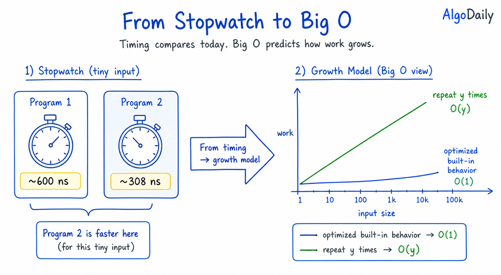
Let's say that the custom_power function took around 600 nanoseconds to execute. We can now compare with program 2.

Program 2:

Let’s now use the Python’s built-in pow function to raise 3 to the power 4 and see how much time it ultimately takes.

```python
from timeit import timeit

t = timeit("pow(3, 4)")
print(t)
```
```js
var start = new Date().getTime();
console.log(Math.pow(3, 4));
var end = new Date().getTime();

console.log(`Call to customPower took ${end - start} milliseconds`);
```
```java
import java.lang.Math;

public class Main {
    public static void main(String[] args) {
        long startTime = System.nanoTime();
        System.out.println(Math.pow(3, 4));
        long endTime = System.nanoTime();

        long duration = endTime - startTime;
        System.out.println(duration + " nanoseconds");
    }
}
```
```cpp
#include <iostream>
#include <chrono>
#include <cmath>

int main() {
    auto start = std::chrono::high_resolution_clock::now();
    std::cout << std::pow(3, 4) << std::endl;
    auto end = std::chrono::high_resolution_clock::now();

    auto duration = std::chrono::duration_cast<std::chrono::nanoseconds>(end - start);
    std::cout << duration.count() << " nanoseconds" << std::endl;
    return 0;
}
```
```csharp
using System;
using System.Diagnostics;

class Program {
    static void Main(string[] args) {
        Stopwatch stopwatch = new Stopwatch();
        stopwatch.Start();
        Console.WriteLine(Math.Pow(3, 4));
        stopwatch.Stop();

        Console.WriteLine($"{stopwatch.Elapsed.TotalMilliseconds} milliseconds");
    }
}
```
```go
package main

import (
	"fmt"
	"math"
	"time"
)

func main() {
	start := time.Now();
	fmt.Println(math.Pow(3, 4));
	end := time.Now();

	duration := end.Sub(start);
	fmt.Println(duration.Nanoseconds(), "nanoseconds");
}
```

Step Six

Again, you'll see the time taken to execute. The results are as follows.

308 ns ± 5.03 ns per loop (mean ± std. dev. of 7 runs, 1000000 loops each)

Call to customPower took 7 miliseconds

1555964 nanoseconds

8.11 miliseconds

51607 nanoseconds

51607 nanoseconds

Step Seven

Please note that the built-in function took around 308 nanoseconds.

What does this mean?

You can clearly see that Program 2 is twice as fast as Program 1. This is just a simple example. However if you are building a real-world application, the wrong choice of algorithms can result in sluggish and inefficient user experiences. Thus, it is very important to determine algorithm complexity and optimize for it.

Timing Vs Growth

The built-in pow call was faster in the measurement, but Big O is not mainly about one stopwatch result.

In interviews, the bigger question is: how does the work scale as the input grows? A faster constant-time library call and a repeated loop may look close for tiny inputs, but their growth patterns can separate quickly.

Timing Vs Growth

Big(O) Notation

Let's now talk about Big(O) Notation. Given what we've seen, you may ask-- why do we need Big O if we can just measure execution speed?

In the last section, we recorded the clock time that our computer took to execute a function. We then used this clock time to compare the two programs. But clock time is hardware dependent. An efficient program may take more time to execute on a slower computer than an inefficient program on a fast computer.

So clock time is not a good metric to find time complexity. Then how do we compare the algorithm complexity of two programs in a standardized manner? The answer is Big(O) notation.

Big(O) notation is an algorithm complexity metric. It defines the relationship between the number of inputs and the steps taken by the algorithm to process those inputs. Read the last sentence very carefully-- it takes a while to understand. Big(O) is NOT about measuring speed, it is about measuring the amount of work a program has to do as an input scales.

We can use Big(O) to define both time and space complexity. The below are some of the examples of Big(O) notation, starting from "fastest"/"best" to "slowest"/"worst".

Function Big(O) Notation Constant O(c) Logarithmic O(log(n)) Linear O(n) Quadratic O(n^2) Cubic O(n^3) Exponential O(2^n) Factorial O(n!)

Let’s see how to calculate time complexity for some of the aforementioned functions using Big(O) notation.

Simplifying Big(O)

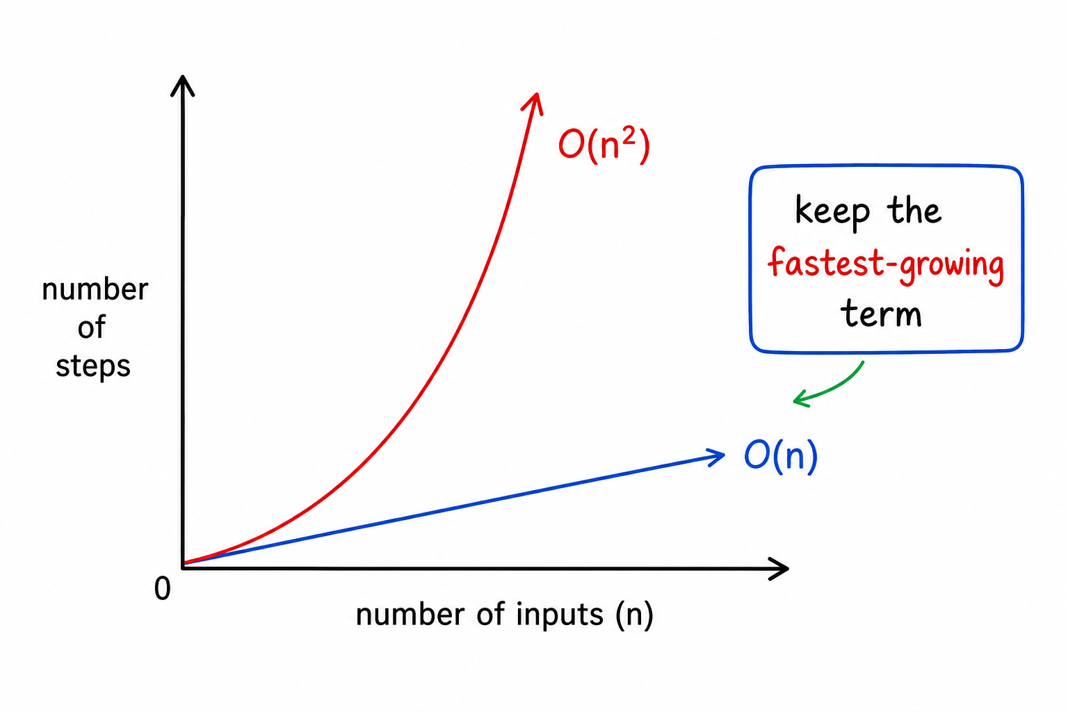
When we write Big(O), we usually care about how the algorithm grows as the input gets very large.

Because of that, we simplify the expression by keeping the part that grows the fastest.

For example:

Step Count Big(O) 5 O(1) 2n O(n) n + 20 O(n) n² + n O(n²) 3n² + 10n + 50 O(n²)

This is why constants and smaller terms are usually dropped. They may affect the actual runtime on a real machine, but they do not change the long-term growth pattern.

Here is a simple example:

Simplifying Big(O)

```python
def print_pairs_and_items(items):
    # Runs n times
    for item in items:
        print(item)

    # Runs n * n times
    for first in items:
        for second in items:
            print(first, second)
```

The first loop is `O(n)`, and the nested loop is `O(n²)`.

Together, the total is `O(n + n²)`, which simplifies to `O(n²)`.

Dominant Term Check

If an algorithm performs 3n² + 5n + 10 steps, what Big(O) time complexity should we usually report?

Multiple Choice

Select the best time complexity from following options.

Constant Complexity

Big(O) Notation for Time Complexity

In this section we will see examples of finding the Big(O) notation for certain constant, linear and quadratic functions.

Constant Complexity

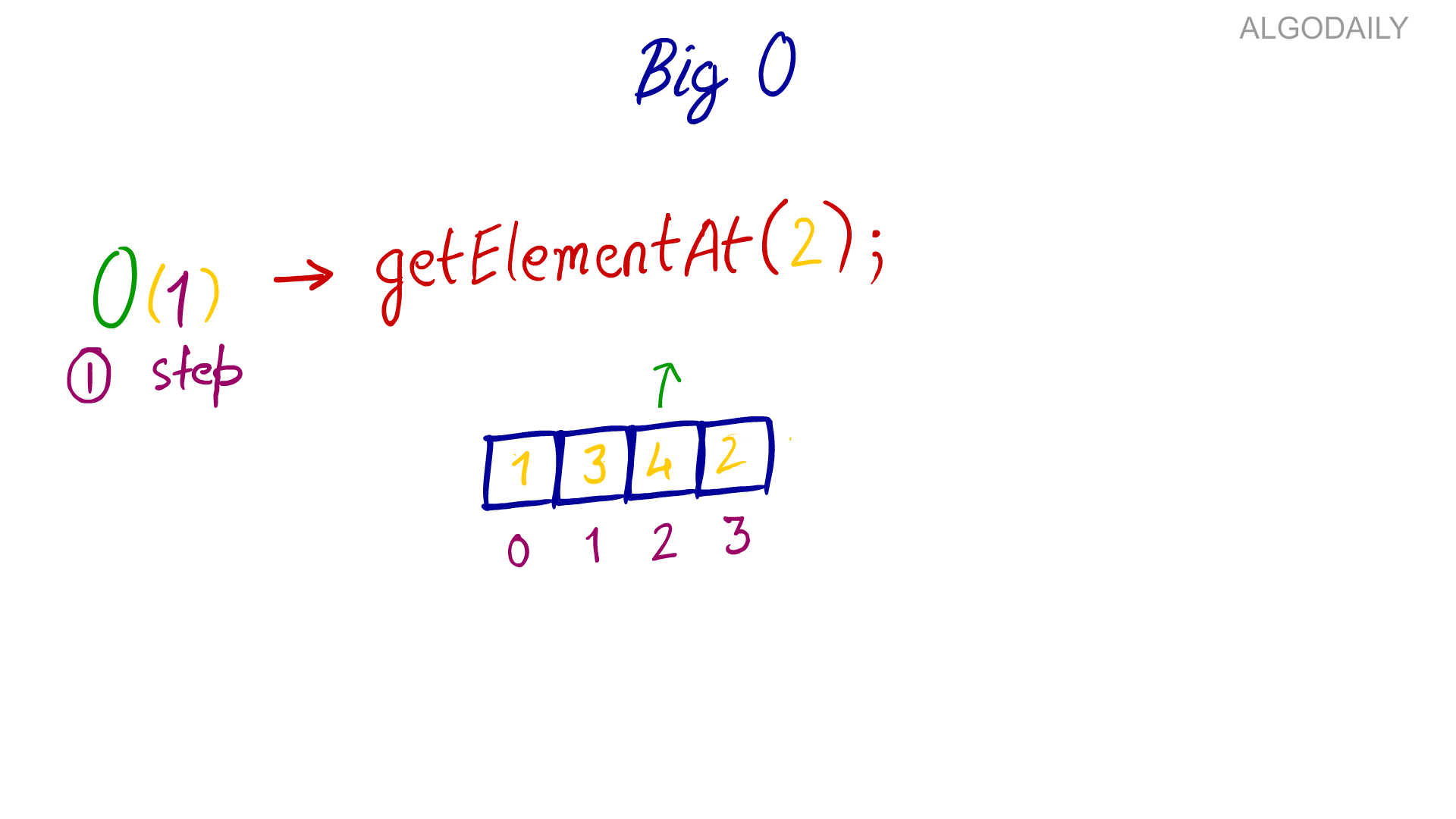
In the constant complexity, the steps taken to complete the execution of a program remains the same irrespective of the input size. Look at the following example:

```python
def display_first_cube(items):
    result = pow(items[0],3)
    print (result)

inputs = [2, 3, 4, 5, 6, 7]
display_first_cube(inputs)
```
```js
function displayFirstCube(items) {
    const result = Math.pow(items[0], 3);
    console.log(result);
}

const inputs = [2, 3, 4, 5, 6, 7];
displayFirstCube(inputs);
```
```java
import java.lang.Math;

public class Main {
    public static void displayFirstCube(int[] items) {
        double result = Math.pow(items[0], 3);
        System.out.println(result);
    }

    public static void main(String[] args) {
        int[] inputs = { 2, 3, 4, 5, 6, 7 };
        displayFirstCube(inputs);
    }
}
```
```cpp
#include <iostream>
#include <cmath>

void displayFirstCube(int items[], int size) {
    double result = std::pow(items[0], 3);
    std::cout << result << std::endl;
}

int main() {
    int inputs[] = {2, 3, 4, 5, 6, 7};
    displayFirstCube(inputs, sizeof(inputs)/sizeof(inputs[0]));
    return 0;
}
```
```csharp
using System;

class Program {
    public static void DisplayFirstCube(int[] items) {
        double result = Math.Pow(items[0], 3);
        Console.WriteLine(result);
    }

    static void Main(string[] args) {
        int[] inputs = { 2, 3, 4, 5, 6, 7 };
        DisplayFirstCube(inputs);
    }
}
```
```go
package main

import (
	"fmt"
	"math"
)

func displayFirstCube(items []int) {
	result := math.Pow(float64(items[0]), 3)
	fmt.Println(result)
}

func main() {
	inputs := []int{2, 3, 4, 5, 6, 7}
	displayFirstCube(inputs)
}
```

Step Ten

In the above example, the display_first_cube element calculates the cube of a number. That number happens to be the first item of the list that passed to it as a parameter. No matter how many elements there are in the list, the display_first_cube function always performs two steps. First, calculate the cube of the first element. Second, print the result on the console. Hence the algorithm complexity remains constant (it does not scale with input).

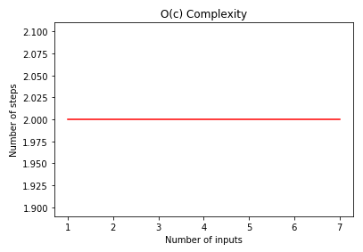
Let’s plot the constant algorithm complexity.

```python
import numpy as np
import matplotlib.pyplot as plt

num_of_inputs = np.array([1,2,3,4,5,6,7])
steps = [2 for n in num_of_inputs]
 
plt.plot(num_of_inputs, steps, 'r')
plt.xlabel('Number of inputs')
plt.ylabel('Number of steps')
plt.title('O(c) Complexity')

plt.show()

# No matplotlib support in this terminal.
# Go to the next screen for the results!
```

Step Eleven

In the above code we have a list num_of_inputs that contains a different number of inputs. The steps list will always contain 2 for each item in the num_of_inputs list. If you plot the num_of_inputs list on x-axis and the steps list on y-axis you will see a straight line as shown in the output:

Linear Complexity*

In functions or algorithms with linear complexity, a single unit increase in the input causes a unit increase in the steps required to complete the program execution.

A function that calculates the cubes of all elements in a list has a linear complexity. This is because as the input (the list) grows, it will need to do one unit more work per item. Look at the following script.

```python
def display_all_cubes(items):
    for item in items:
        result = pow(item,3)
        print (result)

inputs = [2,3,4,5,6,7]
display_all_cubes(inputs)
```
```js
function displayAllCubes(items) {
    for (let item of items) {
        const result = Math.pow(item, 3);
        console.log(result);
    }
}


const inputs = [2, 3, 4, 5, 6, 7];
displayAllCubes(inputs);
```
```java
import java.lang.Math;

public class Main {
    public static void displayAllCubes(int[] items) {
        for (int i = 0; i < items.length; i++) {
            double result = Math.pow(items[i], 3);
            System.out.println(result);
        }
    }

    public static void main(String[] args) {
        int[] inputs = { 2, 3, 4, 5, 6, 7 };
        displayAllCubes(inputs);
    }
}
```
```cpp
#include <iostream>
#include <cmath>

void displayFirstCube(int items[], int size) {
    double result = std::pow(items[0], 3);
    std::cout << result << std::endl;
}

int main() {
    int inputs[] = {2, 3, 4, 5, 6, 7};
    displayFirstCube(inputs, sizeof(inputs)/sizeof(inputs[0]));
    return 0;
}
```
```csharp
using System;

class Program {
    public static void DisplayFirstCube(int[] items) {
        double result = Math.Pow(items[0], 3);
        Console.WriteLine(result);
    }

    static void Main(string[] args) {
        int[] inputs = { 2, 3, 4, 5, 6, 7 };
        DisplayFirstCube(inputs);
    }
}
```
```go
package main

import (
	"fmt"
	"math"
)

func displayFirstCube(items []int) {
	result := math.Pow(float64(items[0]), 3)
	fmt.Println(result)
}

func main() {
	inputs := []int{2, 3, 4, 5, 6, 7}
	displayFirstCube(inputs)
}
```

Step Thirteen

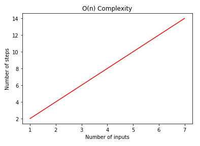
For each item in the items list passed as a parameter to display_all_cubes function, the function finds the cube of the item and then displays it on the screen. If you double the elements in the input list, the steps needed to execute the display_all_cubes function will also be doubled. For the functions, with linear complexity, you should see a straight line increasing in positive direction as shown below:

```python
import numpy as np
import matplotlib.pyplot as plt

num_of_inputs = np.array([1,2,3,4,5,6,7])
steps = [2*n for n in num_of_inputs]

plt.plot(num_of_inputs, steps, 'r')
plt.xlabel('Number of inputs')
plt.ylabel('Number of steps')
plt.title('O(n) Complexity')
plt.show()

# No matplotlib support in this terminal.
# Go to the next screen for the results!
```

Quadratic Complexity

As you might guess by now-- in a function with quadratic complexity, the output steps increase quadratically with the increase in the inputs. Have a look at the following example:

```python
def display_all_products(items):
    for item in items:
        for inner_item in items:
            print(item * inner_item)

inputs = [2, 3, 4, 5 ,6]
display_all_products(inputs)
```
```js
function displayAllProducts(items) {
    for (let item of items) {
        for (let innerItem of items) {
            const result = item * innerItem;
            console.log(result);
        };
    }
}


const inputs = [2, 3, 4, 5, 6, 7];
displayAllProducts(inputs);
```
```java
import java.lang.Math;

public class Main {
    public static void displayAllProducts(int[] items) {
        for (int i = 0; i < items.length; i++) {
            for (int j = 0; j < items.length; j++) {
                int result = items[i] * items[j];
                System.out.println(result);
            }
        }
    }

    public static void main(String[] args) {
        int[] inputs = { 2, 3, 4, 5, 6, 7 };
        displayAllProducts(inputs);
    }
}
```
```cpp
#include <iostream>

void displayAllProducts(int items[], int size) {
    for (int i = 0; i < size; i++) {
        for (int j = 0; j < size; j++) {
            int result = items[i] * items[j];
            std::cout << result << std::endl;
        }
    }
}

int main() {
    int inputs[] = {2, 3, 4, 5, 6, 7};
    displayAllProducts(inputs, sizeof(inputs)/sizeof(inputs[0]));
    return 0;
}
```
```csharp
using System;

class Program {
    public static void DisplayAllProducts(int[] items) {
        foreach (int item in items) {
            foreach (int innerItem in items) {
                int result = item * innerItem;
                Console.WriteLine(result);
            }
        }
    }

    static void Main(string[] args) {
        int[] inputs = { 2, 3, 4, 5, 6, 7 };
        DisplayAllProducts(inputs);
    }
}
```
```go
package main

import (
	"fmt"
)

func displayAllProducts(items []int) {
	for _, item := range items {
		for _, innerItem := range items {
			result := item * innerItem
			fmt.Println(result)
		}
	}
}

func main() {
	inputs := []int{2, 3, 4, 5, 6, 7}
	displayAllProducts(inputs)
}
```

Step Fifteen

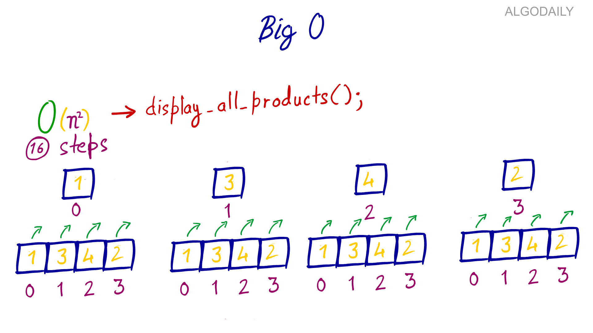
In the above code, the display_all_products function multiplies each item in the “items” list with all the other elements.

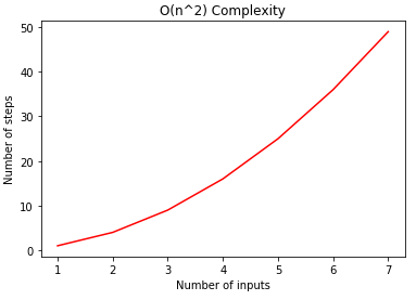
The outer loop iterates through each item, and then for each item in the outer loop, the inner loop iterates over each item. This makes total number of steps n x n where n is the number of items in the “items” list.

If you plot the inputs and the output steps, you should see the graph for a quadratic equation as shown below. Here is the output:

```python
import numpy as np
import matplotlib.pyplot as plt

num_of_inputs = np.array([1,2,3,4,5,6,7])
steps = [pow(n,2) for n in num_of_inputs]

plt.plot(num_of_inputs, steps, 'r')
plt.xlabel('Number of inputs')
plt.ylabel('Number of steps')
plt.title('O(n^2) Complexity')
plt.show()

# No matplotlib support in this terminal.
# Go to the next screen for the results!
```

Fill In

The time complexity of the following code is:

function until(num) {
    let i = num;
    while (i > 0) {
        console.log(i);
        i -= 1;
    }
}

console.log(until(10));

def until(num):
    i = num
    while i > 0:
        print(i)
        i -= 1

print(until(10))

Big(O) Notation For Space Complexity

Big(O) Notation for Space Complexity

To find space complexity, we simply calculate the space (working storage, or memory) that the algorithm will need to allocate against the items in the inputs. Let’s again take a look at the display_first_cube function.

```python
def display_first_cube(items):
    result = pow(items[0],3)
    print (result)

inputs = [2, 3, 4, 5, 6, 7]
display_first_cube(inputs)
```
```js
function displayFirstCube(items) {
    const result = Math.pow(items[0], 3);
    console.log(result);
}

const inputs = [2, 3, 4, 5, 6, 7];
displayFirstCube(inputs);
```
```java
import java.lang.Math;

public class Main {
    public static void displayFirstCube(int[] items) {
        double result = Math.pow(items[0], 3);
        System.out.println(result);
    }

    public static void main(String[] args) {
        int[] inputs = { 2, 3, 4, 5, 6, 7 };
        displayFirstCube(inputs);
    }
}
```
```cpp
#include <iostream>
#include <cmath>

void displayFirstCube(int items[], int size) {
    double result = std::pow(items[0], 3);
    std::cout << result << std::endl;
}

int main() {
    int inputs[] = {2, 3, 4, 5, 6, 7};
    displayFirstCube(inputs, sizeof(inputs)/sizeof(inputs[0]));
    return 0;
}
```
```csharp
using System;

class Program {
    public static void DisplayFirstCube(int[] items) {
        double result = Math.Pow(items[0], 3);
        Console.WriteLine(result);
    }

    static void Main(string[] args) {
        int[] inputs = { 2, 3, 4, 5, 6, 7 };
        DisplayFirstCube(inputs);
    }
}
```
```go
package main

import (
	"fmt"
	"math"
)

func displayFirstCube(items []int) {
	result := math.Pow(float64(items[0]), 3)
	fmt.Println(result)
}

func main() {
	inputs := []int{2, 3, 4, 5, 6, 7}
	displayFirstCube(inputs)
}
```

Space Complexity Comparison

Here no matter the size of the input, the display_first_cube has to allocate memory only once for the result variable. Hence the Big(O) notation for the space complexity of the “display_first_cube” will be O(1) which is basically O(c) i.e. constant.

Similarly, the space complexity of the display_all_cubes function will be O(n) since for each item in the input, space has to be allocated in memory.

Best Vs Worst Case Complexity

Best vs. Worst Case Complexity

You may hear the term "worst case" being used when discussing complexities.

An algorithm can have two types of complexities. They are best case scenarios and worst case scenarios.

The best case complexity refers to the complexity of an algorithm in the ideal situation. For instance, if you want to search an item X in a list of N items-- the best case scenario is that we find the item at the first index, in which case the algorithm complexity will be O(1).

The worst case is that we find the item at the nth (or last) index, in which case the algorithm complexity would be be O(n) (where n is the total number of items in the list). When we use the term "algorithmic complexity", we generally refer to the worst case complexity. This is to ensure that we are optimizing for the least ideal situation.

Memory And Cases

We’ve now separated two dimensions of complexity:

Time: how many steps the algorithm may take.
Space: how much extra memory it allocates.

Then we ask about the scenario: best case tells us the lucky path, while worst case tells us what we must be prepared to handle.

Memory And Cases

Fill In

Sorting an integer array of consecutive elements is an example of ___ case time complexity.

Conclusion

Algorithm complexity is used to measure the performance of an algorithm in terms of time taken and the space consumed.

Big(O) notation is one of the most commonly used metrics for measuring algorithm complexity. In this article you saw how to find different types of time and space complexities of algorithms using Big(O) notation. You'll now be better equipped to make trade-off decisions based on complexity in the future.

True or False

If an algorithm has a time complexity of O(n), it means that the algorithm will always have n nested loops.

One Pager Cheat Sheet

With Algorithm Complexity and Big O Notation, developers can measure the performance of a program, in terms of time and space complexity, to determine the most effective algorithm to use.
Using Program 1 as an example, we can see the importance of ensuring that algorithms are designed to be as efficient as possible to maximize performance.
We can use %timeit in a Jupyter Notebook or language interpreter to measure the performance of an algorithm.
- Count the repeated operations first; runtime measurements are just evidence of that growth pattern.
The program took 600 ns ± 230 ns per loop, 4 milliseconds to call customPower, and 337291 nanoseconds in total.
The built-in pow function took 600 nanoseconds to raise 3 to the power 4, which is substantially less compared to program 2.
The execution time for Python, Javascript, and Java was 308 ns, 7 ms, and 1555964 ns, respectively.
The efficient choice of algorithms can greatly improve user experience, and this is shown by Program 2 being twice as fast as Program 1, taking only 308 nanoseconds.
- Big O abstracts away one machine’s timing and focuses on how work grows with input size.
Big(O) Notation measures the time complexity of an algorithm based on the relationship between the number of inputs and the steps it takes to process them.
- Big(O) keeps the dominant growth term and drops constants or smaller terms.
- For Big(O), 3n² + 5n + 10 is reported as O(n²).
The best complexity metric given is O(log(n)), as it takes logarithmic time in proportion to the input data.
The execution of a program with Constant Complexity remains the same, regardless of the input size.
The display_first_cube function has a constant algorithm complexity which does not scale with input.
Thenum_of_inputson the x-axis and thestepson the y-axis plot out a straight line when graphed.
A function or algorithm with linear complexity will require an equal increase in the number of steps required for execution as the number of units in its input increases.
The display_all_cubes function has linear complexity and its execution time increases proportionally with the number of items in the items list.
The complexity of a function increases quadratically as the input size increases.
The display_all_products function in the code iterates through n items in a n x n loop and outputs a graph showing the quadratic equation.
The space complexity of an algorithm can be determined by calculating the memory needed to store its inputs, expressed in terms of Big(O) Notation.
The space complexity of the display_first_cube is O(1) (constant), while that of the display_all_cubes is O(n).
The complexity of an algorithm can be defined as its worst case scenario, which is optimized for the least ideal situation.
- Complexity usually means worst-case time or space growth unless stated otherwise.
Sorting an array with consecutive elements is a best case scenario, requiring O(n) operations.
Measuring algorithm performance in terms of time taken and space consumed can be done through Big(O) notation.
No, O(n) time complexity does not necessarily mean that the algorithm will use n nested loops.

Open interactive view →