Graph Algorithms: Shortest Path and Connectivity

Why this lesson matters

Now that you've covered Intermediate Data Structures: Trees and Graphs and practiced BFS/DFS, we can ask more interview-shaped graph questions:

• What is the shortest route from one node to another?
• Which nodes belong to the same connected component?
• When should we use BFS, Dijkstra's algorithm, or a connectivity structure?

This lesson is not about memorizing every graph algorithm. In a 30-day crash course, the win is learning the decision rules that let you choose the right tool quickly.

By the end, you should be able to look at a graph prompt and ask: Are the edges weighted? Are weights non-negative? Do I need one path, all distances, or just connected groups?

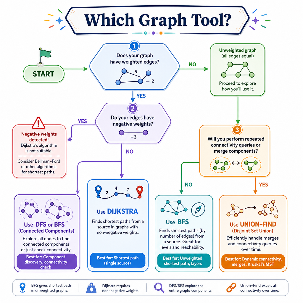
The graph decision checklist

You already know from the graph representation lesson that we usually store graphs as an adjacency list. The next question is what the edges mean.

Use this quick rule set:

Problem shape Best first tool Unweighted shortest path BFS Weighted, non-negative shortest path Dijkstra Count groups / reachable nodes DFS or BFS Many repeated connected? questions Union-Find

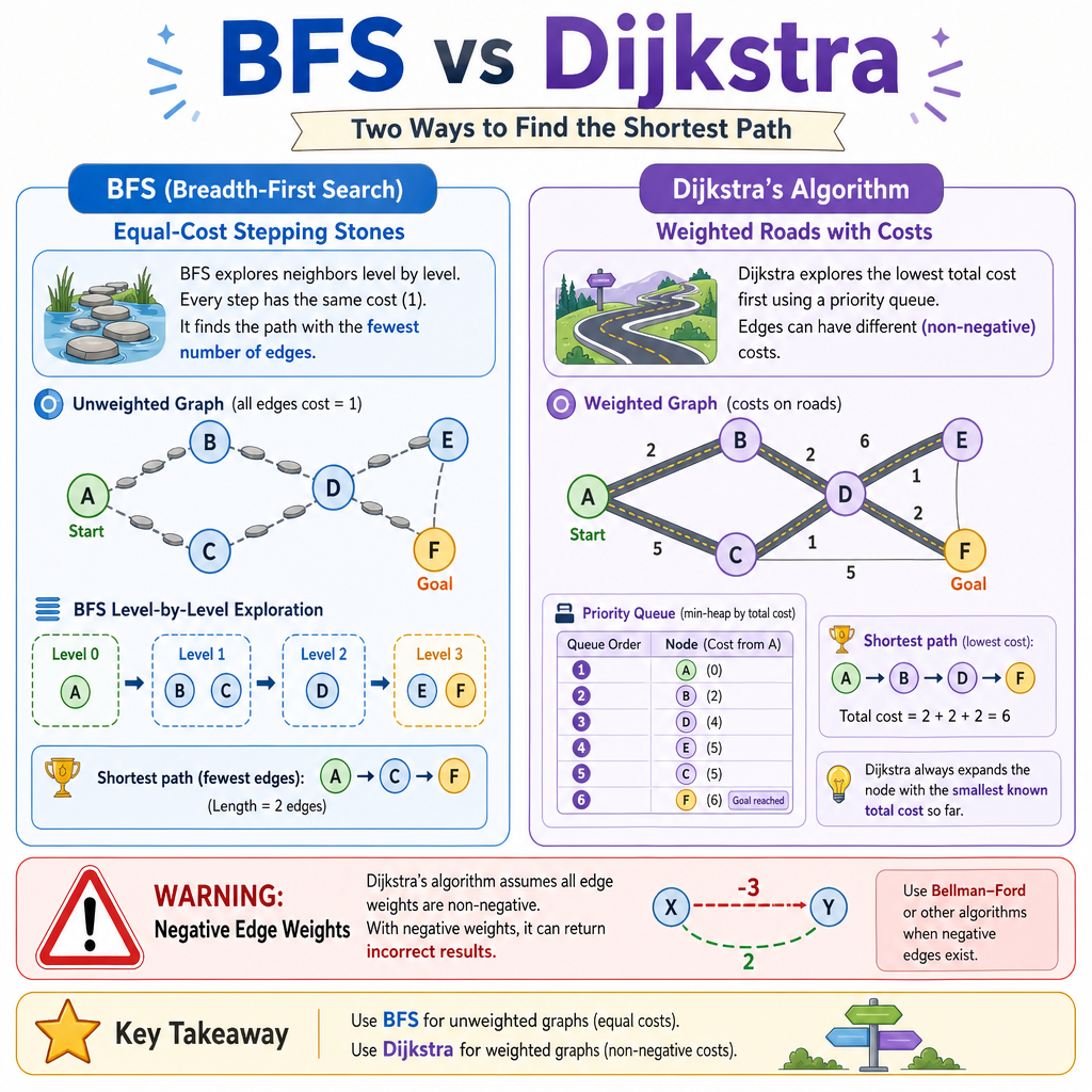
The biggest beginner trap is using DFS for shortest path just because it can reach the target. DFS finds a path. BFS finds the shortest path when every edge has equal cost.

Think of BFS as expanding rings from the start node:

start -> distance 0
neighbors -> distance 1
neighbors of neighbors -> distance 2

The first time BFS reaches a node, it has used the fewest edges possible.

Shortest path with equal edge cost

If every move costs the same, BFS is the shortest-path engine.

Common interview examples:

• shortest path in a grid maze
• minimum number of word transformations
• fewest flights when every flight counts as one hop
• shortest route in an unweighted social network

The key invariant:

When BFS first removes a node from the queue, we have found its shortest distance from the start.

Here is a compact path reconstruction example. Notice that parent lets us rebuild the actual route, not just the distance.

```python
from collections import deque


def shortest_path_unweighted(graph, start, target):
    queue = deque([start])
    parent = {start: None}

    while queue:
        node = queue.popleft()
        if node == target:
            break

        for neighbor in graph[node]:
            if neighbor not in parent:
                parent[neighbor] = node
                queue.append(neighbor)

    if target not in parent:
        return None

    path = []
    cur = target
    while cur is not None:
        path.append(cur)
        cur = parent[cur]

    return path[::-1]


graph = {
    "A": ["B", "C"],
    "B": ["A", "D"],
    "C": ["A", "D", "E"],
    "D": ["B", "C", "F"],
    "E": ["C", "F"],
    "F": ["D", "E"]
}

print(shortest_path_unweighted(graph, "A", "F"))
```

You are given an unweighted graph where each edge represents one move. You need the minimum number of moves from start to target.

Which approach should you reach for first?

When edges have different costs

BFS assumes every edge has the same cost. If one road takes 2 minutes and another takes 20 minutes, we need a different strategy.

Dijkstra's algorithm finds shortest distances from a start node when all edge weights are non-negative.

The mental model:

1. Keep the best known distance to each node.
2. Always expand the currently cheapest unprocessed option.
3. Use a min-heap so the cheapest option is quick to retrieve.
4. Ignore stale heap entries when a better distance has already been found.

This builds directly on the heapq work from Advanced Data Structures: Heaps and Hash Tables.

```python
import heapq


def dijkstra(graph, start):
    distances = {node: float("inf") for node in graph}
    distances[start] = 0
    heap = [(0, start)]

    while heap:
        current_dist, node = heapq.heappop(heap)

        if current_dist > distances[node]:
            continue

        for neighbor, weight in graph[node]:
            new_dist = current_dist + weight
            if new_dist < distances[neighbor]:
                distances[neighbor] = new_dist
                heapq.heappush(heap, (new_dist, neighbor))

    return distances


graph = {
    "A": [("B", 4), ("C", 1)],
    "B": [("D", 1)],
    "C": [("B", 2), ("D", 5)],
    "D": []
}

print(dijkstra(graph, "A"))
```

In Python, Dijkstra's algorithm commonly uses the built-in min-heap module named _____.

Know when not to use it

Dijkstra is powerful, but it has boundaries.

Use Dijkstra when:

• edges have weights
• weights are non-negative
• you need shortest distance from one source to many nodes, or one source to one target

Be careful when:

• the graph has negative edge weights
• the prompt asks for all-pairs shortest paths
• the graph is actually unweighted, where BFS is simpler

Typical complexity with an adjacency list and heap:

O((V + E) log V)

Where:

• V = number of vertices/nodes
• E = number of edges

For this crash course, focus on the practical trigger: weighted non-negative shortest path means Dijkstra is a strong candidate.

When the question is about groups

Not every graph problem asks for a shortest path. Sometimes it asks:

• How many friend circles are there?
• How many islands are in a grid?
• Are all rooms reachable?
• Which servers are in the same network cluster?

That is a connectivity problem.

The pattern is simple:

1. Maintain a visited set.
2. Start a DFS or BFS from each unvisited node.
3. Each traversal marks one complete component.
4. Count how many times you start a new traversal.

This uses the traversal skills from Intermediate Data Structures: Trees and Graphs, but now the purpose is classification into groups.

```python

def count_components(graph):
    visited = set()

    def dfs(node):
        visited.add(node)
        for neighbor in graph[node]:
            if neighbor not in visited:
                dfs(neighbor)

    components = 0
    for node in graph:
        if node not in visited:
            components += 1
            dfs(node)

    return components


graph = {
    0: [1],
    1: [0, 2],
    2: [1],
    3: [4],
    4: [3],
    5: []
}

print(count_components(graph))
```

True or false: In an unweighted graph, the first time BFS discovers a node, it has found the shortest path to that node in number of edges.

When many connectivity questions arrive

DFS/BFS is great when you need to explore a graph once. But if the problem repeatedly asks questions like:

After connecting a and b, are x and y in the same group?

Then repeated graph traversals can become expensive.

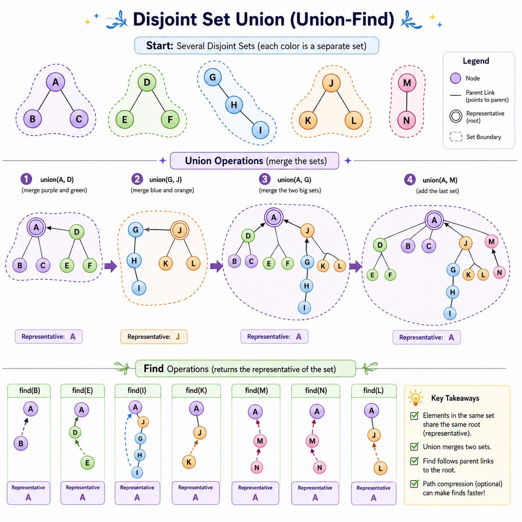
That is where Union-Find, also called Disjoint Set Union, becomes useful.

It supports two ideas:

• find(x): identify the group representative for x
• union(a, b): merge the groups containing a and b

You do not need to over-focus on the internals today. The interview trigger is enough: many merge operations plus many same-group checks usually points to Union-Find.

Your 2-day review loop

To get proficient quickly, revisit graph patterns in short cycles rather than doing one long session and moving on.

Practice set for today:

1. Unweighted shortest path: solve with BFS and reconstruct the path.
2. Weighted shortest path: implement Dijkstra with heapq.
3. Connected components: count groups with DFS or BFS.
4. Connectivity checks: identify when Union-Find would be better than repeated traversal.

Review again in 2 days:

• Re-code BFS shortest path from memory.
• Re-code Dijkstra's loop without looking.
• Explain why DFS is not enough for shortest path in an unweighted graph.

Next, we will zoom out into Problem Solving Strategies and Competitive Programming, where choosing the pattern quickly becomes the main skill.