What Is Deep Learning?

Deep Learning Defined

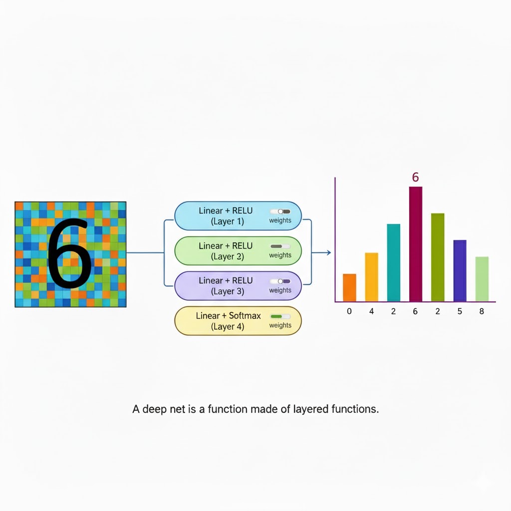
Deep learning is a way to learn functions by stacking layers of simple units (neurons) so that the whole network can approximate very complex input→output mappings. A neural network is just a composable function: output = layer_L(...layer_2(layer_1(input))).

Why “deep”? Because there are many layers (depth). Why “learning”? Because the network’s numeric knobs (its weights and biases) are tuned to minimize a loss—a number that measures how wrong the network is on your data.

Where It Fits

• Machine learning (ML): learn patterns from data.
• Representation learning: learn useful features automatically (instead of hand-crafting them).
• Deep learning (DL): representation learning with many layers of differentiable transformations.

DL shines when you have large datasets, high-dimensional inputs (images, audio, text), and the need for end-to-end learning.

From Perceptron to Neuron

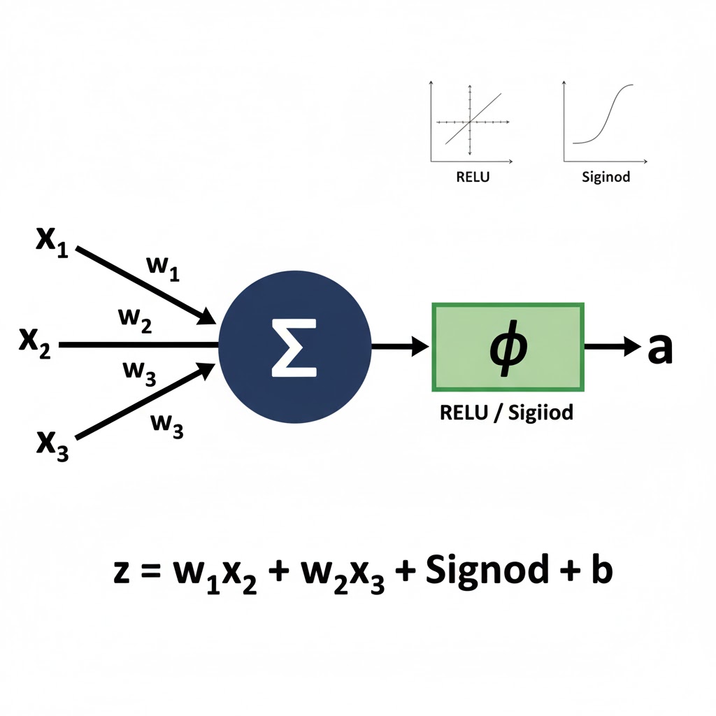
A perceptron is a mathematical model of a biological neuron that takes numerical inputs, applies weights, adds a bias, and uses an activation function to produce a binary output, classifying data into two categories.

The original perceptron computed: y = step(w·x + b). Modern neurons do: z = w·x + b, then a = φ(z) where φ is an activation function (e.g., ReLU, sigmoid, tanh). Stacking many neurons gives you a layer; stacking layers gives you a network.

Which statement is most accurate?

The Math You Really Need

Here's the mathematical terms at play:

• Weights (W) and biases (b): the parameters we learn.
• Activation function φ: adds non-linearity (e.g., ReLU(x) = max(0,x)).
• Loss: scalar measuring error, e.g., MSE for regression, cross-entropy for classification.
• Gradient: vector of partial derivatives that tells us how to tweak parameters to reduce loss.
• Gradient descent: update rule θ ← θ − η ∇θ L with learning rate η.

A Tiny Neuron

Here is a tiny neuron implementation. It is a single neuron with ReLU activation, trained with plain gradient descent to learn y ≈ 2*x + 1 on synthetic data. Standard library only.

```python
import random
import math

def relu(x):
    return x if x > 0 else 0.0

def relu_grad(x):
    return 1.0 if x > 0 else 0.0

def train_single_neuron(epochs=2000, lr=0.01, seed=42):
    random.seed(seed)
    # Generate simple 1D data: y = 2x + 1 + noise
    xs = [random.uniform(-2.0, 2.0) for _ in range(200)]
    ys = [2.0 * x + 1.0 + random.gauss(0, 0.1) for x in xs]

    # Parameters of a 1D neuron: w and b
    w = random.uniform(-1.0, 1.0)
    b = 0.0

    for epoch in range(epochs):
        dw = 0.0
        db = 0.0
        loss = 0.0
        for x, y in zip(xs, ys):
            z = w * x + b
            a = relu(z)
            # Mean squared error (per sample)
            diff = a - y
            loss += 0.5 * diff * diff
            # Backprop through ReLU and linear
            da_dz = relu_grad(z)
            dL_dz = diff * da_dz
            dw += dL_dz * x
            db += dL_dz * 1.0

        n = len(xs)
        # Average gradients
        w -= lr * (dw / n)
        b -= lr * (db / n)
        if (epoch + 1) % 200 == 0:
            print(f"epoch={epoch+1:4d} loss={loss/n:.4f} w={w:.3f} b={b:.3f}")

    # Simple driver prediction
    test_x = 1.5
    pred = relu(w * test_x + b)
    print(f"for x={test_x}, prediction≈{pred:.3f} (true≈{2*test_x+1:.3f})")
    return w, b

if __name__ == "__main__":
    train_single_neuron()
```

ReLU(x) = max(0, x) is differentiable everywhere, including at x = 0.

Forward, Loss, Backprop: The Loop

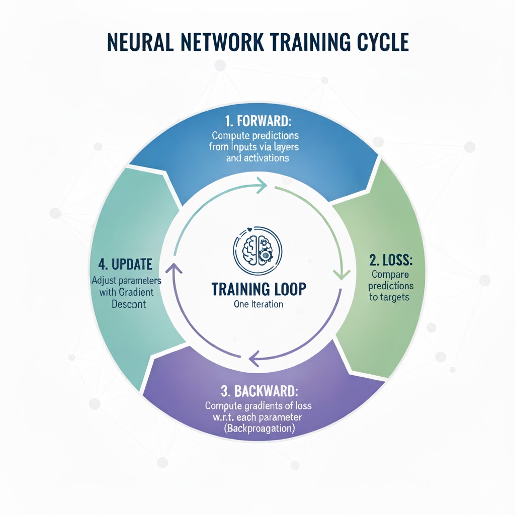
The Forward, Loss, Backprop loop is the core training process for a neural network, where a forward pass makes a prediction, a loss function calculates how wrong it is, and backpropagation computes gradients to update the model's weights, reducing error over many iterations to improve future predictions.

1. Forward: compute predictions from inputs via layers and activations.
2. Loss: compare predictions to targets.
3. Backward: compute gradients of loss w.r.t. each parameter (backpropagation).
4. Update: adjust parameters with gradient descent (or a fancier optimizer).

Put the training steps in the correct order:

Two-Layer Network Implementation

Here is a minimal 2-layer MLP for binary classification on a toy dataset using the standard library only.

```python
import random
import math

def sigmoid(x):  # activation for last layer (probability)
    return 1.0 / (1.0 + math.exp(-x))

def dsigmoid(y):  # derivative given output y = sigmoid(x)
    return y * (1.0 - y)

def relu(x):
    return x if x > 0 else 0.0

def relu_grad(x):
    return 1.0 if x > 0 else 0.0

def dot(a, b):
    return sum(x*y for x, y in zip(a, b))

def matvec(W, v):
    # W: list of rows, v: vector
    return [dot(row, v) for row in W]

def add(v, b):
    return [x + y for x, y in zip(v, b)]

def outer(u, v):
    # returns matrix: u * v^T
    return [[ui * vj for vj in v] for ui in u]

def make_toy_data(n=400, seed=0):
    random.seed(seed)
    # Two Gaussian blobs in 2D
    X, Y = [], []
    for _ in range(n//2):
        X.append([random.gauss(-1.0, 0.5), random.gauss(0.0, 0.5)])
        Y.append(0.0)
    for _ in range(n//2):
        X.append([random.gauss(1.0, 0.5), random.gauss(0.0, 0.5)])
        Y.append(1.0)
    # Shuffle
    idx = list(range(n))
    random.shuffle(idx)
    X = [X[i] for i in idx]
    Y = [Y[i] for i in idx]
    return X, Y

def train_mlp(epochs=1000, lr=0.05, hidden=8):
    X, Y = make_toy_data()

    # Initialize params
    input_dim = 2
    W1 = [[random.uniform(-0.5, 0.5) for _ in range(input_dim)] for _ in range(hidden)]
    b1 = [0.0 for _ in range(hidden)]
    W2 = [random.uniform(-0.5, 0.5) for _ in range(hidden)]  # row vector
    b2 = 0.0

    for epoch in range(epochs):
        total_loss = 0.0
        # accumulate gradients (batch GD for clarity)
        dW1 = [[0.0]*input_dim for _ in range(hidden)]
        db1 = [0.0]*hidden
        dW2 = [0.0]*hidden
        db2 = 0.0

        for x, y in zip(X, Y):
            # Forward
            z1 = add(matvec(W1, x), b1)          # hidden pre-activation
            a1 = [relu(z) for z in z1]           # hidden activation
            z2 = dot(W2, a1) + b2                # scalar
            a2 = sigmoid(z2)                     # probability

            # Loss: binary cross-entropy
            # add tiny epsilon for stability
            eps = 1e-8
            loss = -(y*math.log(a2+eps) + (1-y)*math.log(1-a2+eps))
            total_loss += loss

            # Backprop (output)
            dL_da2 = -(y/(a2+eps)) + ((1-y)/(1-a2+eps))
            da2_dz2 = dsigmoid(a2)
            dL_dz2 = dL_da2 * da2_dz2  # scalar

            # Grad for W2, b2, and a1
            for j in range(hidden):
                dW2[j] += dL_dz2 * a1[j]
            db2 += dL_dz2
            da1 = [dL_dz2 * W2[j] for j in range(hidden)]

            # Backprop to layer 1 (through ReLU)
            dz1 = [da1[j] * relu_grad(z1[j]) for j in range(hidden)]
            # Grad for W1 and b1
            for j in range(hidden):
                for i in range(input_dim):
                    dW1[j][i] += dz1[j] * x[i]
                db1[j] += dz1[j]

        n = len(X)
        # Update
        for j in range(hidden):
            for i in range(input_dim):
                W1[j][i] -= lr * (dW1[j][i] / n)
            b1[j] -= lr * (db1[j] / n)
            W2[j]  -= lr * (dW2[j]  / n)
        b2 -= lr * (db2 / n)

        if (epoch+1) % 100 == 0:
            print(f"epoch={epoch+1:4d} loss={total_loss/n:.4f}")

    # Evaluate accuracy
    correct = 0
    for x, y in zip(X, Y):
        z1 = add(matvec(W1, x), b1)
        a1 = [relu(z) for z in z1]
        z2 = dot(W2, a1) + b2
        a2 = sigmoid(z2)
        pred = 1.0 if a2 >= 0.5 else 0.0
        correct += int(pred == y)
    print(f"train accuracy: {correct/len(X):.3f}")

if __name__ == "__main__":
    train_mlp()
```

A function used to map raw logits to probabilities over multiple classes is called ________. It ensures outputs are non-negative and sum to 1.

Multiclass Heads & Cross-Entropy

For K classes, we compute a vector of logits z ∈ ℝ^K, then apply softmax(z)_k = e^{z_k} / Σ_j e^{z_j}. Use cross-entropy loss: L = − Σ_k y_k log(softmax(z)_k) where y is a one-hot label.

Which combination is typical for multiclass classification?

Regularization & Generalization

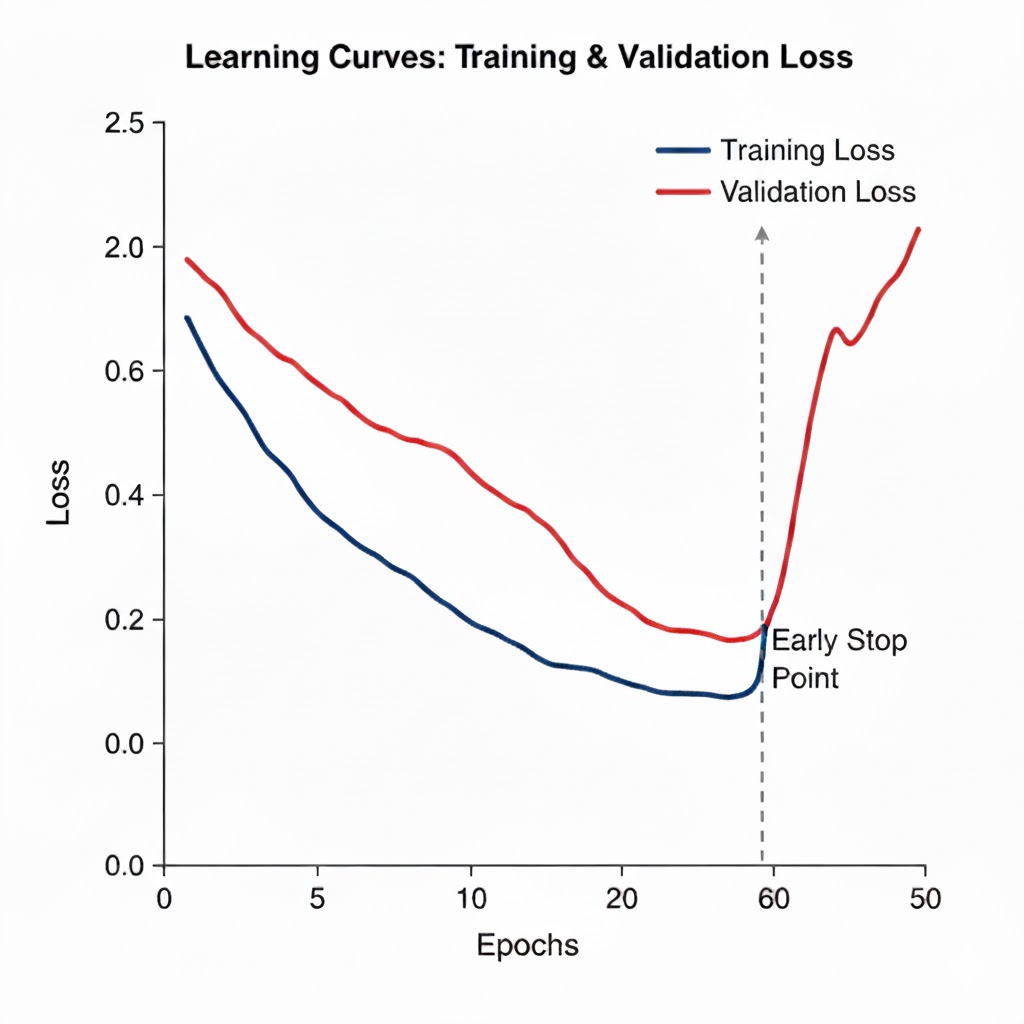
• Overfitting: model learns noise; low training loss, high validation loss.
• Underfitting: model too simple; high training and validation loss.
• Regularization: techniques to improve generalization:

• L2 (weight decay): penalize large weights.
• Early stopping: stop when validation loss worsens.
• Dropout: randomly drop units during training (simulated in code by masking).
• Data augmentation: alter inputs (flips/crops/noise) to create variety.

Add L2 Weight Decay

This illustrates adding L2 penalty to the loss inside training loop.

```python
# Suppose total_loss accumulates data loss already:
# L_total = L_data + (lambda/2) * sum(W^2)

def l2_penalty_mats(mats):
    return sum(sum(w*w for w in row) for M in mats for row in M)

def l2_penalty_vecs(vecs):
    return sum(w*w for v in vecs for w in v) if vecs and isinstance(vecs[0], list) else sum(w*w for w in vecs)

# Example inside training after accumulating gradients:
lam = 1e-3
# add penalty to total_loss (W1,W2 shown)
total_loss += 0.5 * lam * (l2_penalty_mats([W1]) + sum(w*w for w in W2))

# and when updating grads, add lam * W terms (weight decay)
for j in range(hidden):
    for i in range(input_dim):
        dW1[j][i] += lam * W1[j][i]
for j in range(hidden):
    dW2[j] += lam * W2[j]
```

Transformers eliminate the need for recurrence by using attention to connect positions in a sequence directly.

When NOT to Use Deep Learning

• Tiny dataset with easily engineered features? Try simpler ML (like linear or tree-based models).
• Need perfect interpretability or strict guarantees? DL may be harder to justify.
• Low compute budget or latency constraints? A smaller model may be better.

Rule of thumb: start simple, scale up when the problem/data demands it.

Build Your Own MLP

Here's a minimal 2-layer MLP for XOR using standard libraries only.

```javascript
function randu(a, b) { return a + (b - a) * Math.random(); }
function sigmoid(x) { return 1 / (1 + Math.exp(-x)); }
function dsigmoid(y) { return y * (1 - y); }
function relu(x) { return x > 0 ? x : 0; }
function reluGrad(x) { return x > 0 ? 1 : 0; }

function matvec(W, v) {
  const out = new Array(W.length).fill(0);
  for (let r = 0; r < W.length; r++) {
    let s = 0;
    for (let c = 0; c < v.length; c++) s += W[r][c] * v[c];
    out[r] = s;
  }
  return out;
}
function addv(a, b) { return a.map((x, i) => x + b[i]); }

function trainXOR(epochs = 5000, lr = 0.1, hidden = 4) {
  // XOR dataset
  const X = [[0,0],[0,1],[1,0],[1,1]];
  const Y = [0,1,1,0];

  // Params
  const inputDim = 2;
  let W1 = Array.from({length: hidden}, () => Array.from({length: inputDim}, () => randu(-1,1)));
  let b1 = Array.from({length: hidden}, () => 0);
  let W2 = Array.from({length: hidden}, () => randu(-1,1));
  let b2 = 0;

  for (let epoch = 1; epoch <= epochs; epoch++) {
    let dW1 = Array.from({length: hidden}, () => Array(inputDim).fill(0));
    let db1 = Array(hidden).fill(0);
    let dW2 = Array(hidden).fill(0);
    let db2 = 0;
    let loss = 0;

    for (let n = 0; n < X.length; n++) {
      const x = X[n];
      const y = Y[n];

      const z1 = addv(matvec(W1, x), b1);
      const a1 = z1.map(relu);
      const z2 = W2.reduce((s, wj, j) => s + wj * a1[j], b2);
      const a2 = sigmoid(z2);

      // Binary cross-entropy
      const eps = 1e-8;
      loss += -(y*Math.log(a2+eps) + (1-y)*Math.log(1-a2+eps));

      // Backprop
      const dL_da2 = -(y/(a2+eps)) + ((1-y)/(1-a2+eps));
      const dL_dz2 = dL_da2 * dsigmoid(a2);

      for (let j = 0; j < hidden; j++) dW2[j] += dL_dz2 * a1[j];
      db2 += dL_dz2;

      const da1 = W2.map(wj => wj * dL_dz2);
      const dz1 = z1.map((z, j) => da1[j] * reluGrad(z));

      for (let j = 0; j < hidden; j++) {
        for (let i = 0; i < inputDim; i++) dW1[j][i] += dz1[j] * x[i];
        db1[j] += dz1[j];
      }
    }

    const n = X.length;
    for (let j = 0; j < hidden; j++) {
      for (let i = 0; i < inputDim; i++) W1[j][i] -= lr * (dW1[j][i] / n);
      b1[j] -= lr * (db1[j] / n);
      W2[j]  -= lr * (dW2[j]  / n);
    }
    b2 -= lr * (db2 / n);

    if (epoch % 500 === 0) {
      console.log(`epoch=${epoch} loss=${(loss/n).toFixed(4)}`);
    }
  }

  // Driver: predictions
  for (const x of X) {
    const z1 = addv(matvec(W1, x), b1);
    const a1 = z1.map(relu);
    const z2 = W2.reduce((s, wj, j) => s + wj * a1[j], b2);
    const a2 = sigmoid(z2);
    console.log(`x=${x} -> p=${a2.toFixed(3)} -> ${a2>=0.5?1:0}`);
  }
}

if (require.main === module) {
  trainXOR();
}
```

Hardware and Complexity

• Training cost grows with data size, model size, and sequence/image resolution.
• Batch size: how many samples per gradient step. Larger batches use more memory.
• Epoch: one full pass over training data.
• Typical accelerators: GPUs/TPUs; but conceptually all you need is the math we wrote.

Ethics, Safety, and Bias

Neural nets learn what they see. If training data is biased, the model may be biased. Key ideas:

• Dataset curation and evaluation on diverse slices.
• Explainability tools (feature attributions, probes) to audit behavior.
• Safety: avoid harmful outputs; consider rate limits, human review, domain constraints.

Quick Debugging Playbook

• Sanity check: can the model overfit a tiny subset (e.g., 10 samples)?
• Loss not decreasing? Lower lr, check gradient signs and shapes.
• Exploding loss? Clip gradients, reduce lr, check for NaNs.
• Validation worse than training? Add regularization or more data.

Which change most directly combats overfitting?

A single run through the entire training dataset is called an ________.

Without non-linear activations, stacking multiple linear layers is equivalent to a single linear transformation.

You’ve seen what deep learning is, why it works, and you’ve implemented tiny nets from scratch. When you’re ready, port these to a proper framework—but now you’ll know exactly what the framework is doing under the hood.

One Pager Cheat Sheet

• Deep learning learns complex input→output mappings by stacking layers of simple units into a neural network that is a composable function (e.g., output = layer_L(...layer_2(layer_1(input)))), where many layers provide depth and the model’s numeric knobs—the weights and biases—are tuned to minimize a loss.
• Machine learning (ML) learns patterns from data, Representation learning learns useful features automatically, and Deep learning (DL) is representation learning with many layers of differentiable transformations that excels on large datasets, high-dimensional inputs (images, audio, text), and when end-to-end learning is required.
• A perceptron is a mathematical model of a biological neuron that originally produced a binary output via y = step(w·x + b), while modern neurons compute z = w·x + b then a = φ(z) with an activation function (e.g., ReLU, sigmoid, tanh), and stacking layers of such neurons produces neural networks.
• Because the composition of linear maps is itself a linear map, stacking layers that compute z = W x + b (with identity activations) simply collapses to a single equivalent layer with W_eq = W^(L) ... W^(1) and a combined bias, so without a non-linear activation (e.g. ReLU, sigmoid, tanh) depth does not increase a network's representational power and cannot produce non-linear decision boundaries.
• Neural networks learn Weights (W) and biases (b) — the parameters we learn — apply an activation function φ (e.g., ReLU(x) = max(0,x)) to add non-linearity, measure performance with a Loss (e.g., MSE or cross-entropy) as the error measure, compute the Gradient (partial derivatives) as the direction to improve parameters, and use Gradient descent with the update rule θ ← θ − η ∇θ L (step size given by learning rate η) as the update rule.
• A tiny implementation of a single neuron with ReLU activation, trained with gradient descent to learn y ≈ 2*x + 1 on synthetic data, using the standard library only.
• ReLU f(x)=max(0,x) is differentiable for x ≠ 0 but not differentiable at 0 because the left-hand derivative = 0 and the right-hand derivative = 1, though it is continuous at 0, has subgradients in [0,1] there, and is therefore almost everywhere differentiable, so gradient-based training remains practical.
• The core training loop—Forward (compute predictions), Loss (measure error), Backward (compute gradients via backpropagation), and Update (adjust weights using gradient descent or other optimizers)—repeats many times to reduce error and improve the model.
• The steps must occur in order: forward pass to compute y_hat and cache activations, then compute loss to get a scalar L(y_hat, y), then backpropagate gradients to obtain ∂L/∂θ, and finally update parameters with an optimizer (e.g., SGD), because each step depends on the previous step's outputs.
• This is a minimal implementation of a Two-Layer Network: a 2-layer MLP performing binary classification on a toy dataset using the standard library only.
• The missing word is softmax, a mapping from raw logits via p_i = exp(z_i)/sum_j exp(z_j) that produces non-negative outputs which sum to 1 (forming a proper probability distribution), preserves ordering (so the argmax is unchanged), is invariant to additive constants (enabling numerical stability by subtracting max), supports temperature scaling to control peakiness (→ one-hot as temp→0, uniform as temp→∞), reduces to the sigmoid for two classes, and has Jacobian ∂p_i/∂z_j = p_i(δ_ij - p_j) which with cross-entropy and a one-hot target yields the simple gradient p - y.
• Multiclass heads compute a vector of logits z ∈ ℝ^K for K classes, convert them to probabilities with softmax softmax(z)_k = e^{z_k} / Σ_j e^{z_j}, and optimize using cross-entropy loss L = − Σ_k y_k log(softmax(z)_k) where y is a one-hot label.
• The pipeline Linear → softmax → cross-entropy is standard because the final Linear produces unconstrained real-valued logits that softmax turns into a probability distribution, cross-entropy (the negative log-likelihood) trains those probabilities with simple, stable gradients (∂L/∂z = p − y) and a clear probabilistic interpretation with numerically stable fused implementations, while for multi-label problems one should instead use sigmoid + binary cross-entropy.
• Overfitting (low training loss, high validation loss) versus Underfitting (high training and validation loss): Regularization aims to improve generalization using techniques like L2 (weight decay), Early stopping, Dropout, and Data augmentation.
• Add L2 Weight Decay: illustrates adding an L2 penalty to the loss inside the training loop.
• The statement is true: unlike RNN/LSTM models that use recurrence, the transformer uses self-attention—computing queries, keys, and values and weights via softmax(Q K^T / sqrt(d_k)) V—so each layer yields direct, learnable, parallel connections between all positions (thereby eliminating recurrence, providing a short path length for dependencies, and enabling parallel processing across sequence positions), while practical additions like positional encoding, multi-head attention, and masked attention supply order information, richer relations, and autoregressive causality, at the cost of an O(n^2) trade-off in memory and compute.
• For problems with a tiny dataset and easily engineered features try simpler ML (e.g. linear or tree-based models), when you need perfect interpretability or strict guarantees DL is hard to justify, and with low compute or tight latency constraints a smaller model is preferable—start simple and scale up when the problem/data demands it.
• This provides a minimal 2-layer MLP that implements the XOR function using standard libraries only.
• Training cost grows with data size, model size, and sequence/image resolution; Batch size (samples per gradient step) and Epoch (one full pass over data) affect memory and training dynamics, and while typical accelerators are GPUs/TPUs, conceptually you only need the underlying math.
• Neural nets learn what they see, so to mitigate biased training data you should perform dataset curation and evaluation on diverse slices, use explainability tools such as feature attributions and probes to audit behavior, and adopt safety measures like rate limits, human review, and domain constraints to avoid harmful outputs.
• Run a sanity check by confirming the model can overfit a tiny subset (e.g., 10 samples); if loss not decreasing, lower lr and inspect gradients signs/shapes; if exploding loss, clip gradients, reduce lr, and check for NaNs; if validation worse than training, add regularization or gather more data.
• Because Overfitting is primarily a high-variance problem, adding an L2 penalty (a weight decay term like lambda * ||w||^2 that shrinks weights) and using early stopping (monitoring val_loss and halting after patience) both primarily reduce variance—the former by constraining parameter magnitudes and the latter by limiting optimization time—and together act complementarily to improve generalization.
• The correct fill-in is epoch: a single pass through the entire training dataset (aka a pass), which differs from a batch/mini-batch and an iteration—one iteration updates parameters using one batch—and because the number of epochs controls how often the model sees the full data, training for too many epochs can cause overfitting (mitigate with a validation set, early stopping, fewer epochs, or regularization).
• The composition of linear layers of the form f(x) = W x + b is itself a single linear transformation—e.g. f2(f1(x)) = (W2 W1) x + (W2 b1 + b2)—so stacking layers without non-linear activations adds no expressive power, though hidden dimensions can impose a rank constraint on the resulting matrix.
• You’ve learned what deep learning is and why it works, implemented tiny nets from scratch, and are ready to port them to a proper framework—now knowing exactly what the framework is doing under the hood.