Array

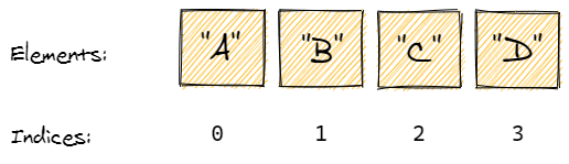
• Quick summary: a collection that stores elements in order and looks them up by index.
• Also known as: fixed array, static array.
• Important facts:
  • Stores elements sequentially, one after another.
  • Each array element has an index. Zero-based indexing is used most often: the first index is 0, the second is 1, and so on.
  • Is created with a fixed size. Increasing or decreasing the size of an array is impossible.
  • Can be one-dimensional (linear) or multi-dimensional.
  • Allocates contiguous memory space for all its elements.
• Pros:
  • Ensures constant time access by index.
  • Constant time append (insertion at the end of an array).
• Cons:
  • Fixed size that can't be changed.
  • Search, insertion and deletion are O(n). After insertion or deletion, all subsequent elements are moved one index further.
  • Can be memory intensive when capacity is underused.
• Notable uses:
  • The String data type that represents text is implemented in programming languages as an array that consists of a sequence of characters plus a terminating character.
• Time complexity (worst case):
  • Access: O(1)
  • Search: O(n)
  • Insertion: O(n) (append: O(1))
  • Deletion: O(n)
• See also:
  • A Gentle Refresher Into Arrays and Strings
  • Interview Problems: Easy Strings
  • Interview Problems: Basic Arrays
  • Interview Problems: Medium Arrays

Arrays are a primitive building block in most languages, here's how to initialize them:

1arr = [1, 2, 3]

xxxxxxxxxx

print(a)

# Python does not have a native support for arrays, but has a List data structure

# which mimicks the behavior of an array. The Python array module requires all

# array elements to be of the same type. We implement our own below.

​

class Array(object):

    """

    sizeOfArray: denotes the total size of the array to be initialized

    arrayType: denotes the data type of the array

    arrayItems: values at each position of array

    """

​

    def __init__(self, sizeOfArray, arrayType=int):

        self.sizeOfArray = len(list(map(arrayType, range(sizeOfArray))))

        self.arrayItems = [arrayType(0)] * sizeOfArray  # initialize array with zeroes

​

    def __str__(self):

        return " ".join([str(i) for i in self.arrayItems])

​

    # function for search

    def search(self, keyToSearch):

        for i in range(self.sizeOfArray):

            if self.arrayItems[i] == keyToSearch:  # brute-forcing

                return i  # index at which element/key was found

​

        return -1  # if key not found, return -1

​

    # function for inserting an element

    def insert(self, keyToInsert, position):

        if self.sizeOfArray > position:

Dynamic array

• Quick summary: an array that can resize itself.
• Also known as: array list, list, growable array, resizable array, mutable array, dynamic table.
• Important facts:
  • Same as array in most regards: stores elements sequentially, uses numeric indexing, allocates contiguous memory space.
  • Expands as you add more elements. Doesn't require setting initial capacity.
  • When it exhausts capacity, a dynamic array allocates a new contiguous memory space that is double the previous capacity, and copies all values to the new location.
  • Time complexity is the same as for a fixed array except for worst-case appends: when capacity needs to be doubled, append is O(n). However, the average append is still O(1).
• Pros:
  • Variable size. A dynamic array expands as needed.
  • Constant time access.
• Cons:
  • Slow worst-case appends: O(n). Average appends: O(1).
  • Insertion and deletion are still slow because subsequent elements must be moved a single index further. Worst-case (insertion into/deletion from the first index, a.k.a. prepending) for both is O(n).
• Time complexity (worst case):
  • Access: O(1)
  • Search: O(n)
  • Insertion: O(n) (append: O(n))
  • Deletion: O(n)
• See also: same as arrays (see above).

xxxxxxxxxx

print(a)

# Python does not have a native support for arrays, but has a List data structure

# which mimicks the behavior of an array. The Python array module requires all

# array elements to be of the same type. We implement our own below.

​

class Array(object):

    """

    sizeOfArray: denotes the total size of the array to be initialized

    arrayType: denotes the data type of the array

    arrayItems: values at each position of array

    """

​

    def __init__(self, sizeOfArray, arrayType=int):

        self.sizeOfArray = len(list(map(arrayType, range(sizeOfArray))))

        self.arrayItems = [arrayType(0)] * sizeOfArray  # initialize array with zeroes

​

    def __str__(self):

        return " ".join([str(i) for i in self.arrayItems])

​

    # function for search

    def search(self, keyToSearch):

        for i in range(self.sizeOfArray):

            if self.arrayItems[i] == keyToSearch:  # brute-forcing

                return i  # index at which element/key was found

​

        return -1  # if key not found, return -1

​

    # function for inserting an element

    def insert(self, keyToInsert, position):

        if self.sizeOfArray > position:

Linked List

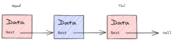
• Quick summary: a linear collection of elements ordered by links instead of physical placement in memory.
• Important facts:
  • Each element is called a node.
    • The first node is called the head.
    • The last node is called the tail.
  • Nodes are sequential. Each node stores a reference (pointer) to one or more adjacent nodes:
    • In a singly linked list, each node stores a reference to the next node.
    • In a doubly linked list, each node stores references to both the next and the previous nodes. This enables traversing a list backwards.
    • In a circularly linked list, the tail stores a reference to the head.
  • Stacks and queues are usually implemented using linked lists, and less often using arrays.
• Pros:
  • Optimized for fast operations on both ends, which ensures constant time insertion and deletion.
  • Flexible capacity. Doesn't require setting initial capacity, can be expanded indefinitely.
• Cons:
  • Costly access and search.
  • Linked list nodes don't occupy continuous memory locations, which makes iterating a linked list somewhat slower than iterating an array.
• Notable uses:
  • Implementation of stacks, queues, and graphs.
• Time complexity (worst case):
  • Access: O(n)
  • Search: O(n)
  • Insertion: O(1)
  • Deletion: O(1)
• See also:
  • What Is the Linked List Data Structure?
  • Implement a Linked List
  • Interview Problems: Linked Lists

xxxxxxxxxx

    linked_list.print_list()

class LinkedListNode:

    def __init__(self, value, next_node=None):

        self.value = value

        self.next_node = next_node

​

    def set_next(self, next_node):

        self.next_node = next_node

​

    def get_next(self):

        return self.next_node

​

    def get_value(self):

        return self.value

​

​

class LinkedList:

    def __init__(self):

        self.head = None

        self.tail = None

​

    def prepend(self, value):

        new_node = LinkedListNode(value)

        new_node.set_next(self.head)

        self.head = new_node

​

        if self.tail is None:

            self.tail = new_node

​

    def append(self, value):

Queue

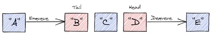
• Quick summary: a sequential collection where elements are added at one end and removed from the other end.
• Important facts:
  • Modeled after a real-life queue: first come, first served.
  • First in, first out (FIFO) data structure.
  • Similar to a linked list, the first (last added) node is called the tail, and the last (next to be removed) node is called the head.
  • Two fundamental operations are enqueuing and dequeuing:
    • To enqueue, insert at the tail of the linked list.
    • To dequeue, remove at the head of the linked list.
  • Usually implemented on top of linked lists because they're optimized for insertion and deletion, which are used to enqueue and dequeue elements.
• Pros:
  • Constant-time insertion and deletion.
• Cons:
  • Access and search are O(n).
• Notable uses:
  • CPU and disk scheduling, interrupt handling and buffering.
• Time complexity (worst case):
  • Access: O(n)
  • Search: O(n)
  • Insertion (enqueuing): O(1)
  • Deletion (dequeuing): O(1)
• See also:
  • Understanding the Queue Data Structure
  • Interview Problems: Queues

xxxxxxxxxx

    print('Queue Size:',myQueue.getSize())

class Queue(object):

    def __init__(self, limit = 10):

        self.queue = []

        self.front = None

        self.rear = None

        self.limit = limit

        self.size = 0

​

    def __str__(self):

        return ' '.join([str(i) for i in self.queue])

​

    # to check if queue is empty

    def isEmpty(self):

        return self.size <= 0

​

    # to add an element from the rear end of the queue

    def enqueue(self, data):

        if self.size >= self.limit:

            return -1          # queue overflow

        else:

            self.queue.append(data)

​

        # assign the rear as size of the queue and front as 0

        if self.front is None:

            self.front = self.rear = 0

        else:

            self.rear = self.size

​

        self.size += 1

Stack

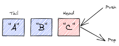
• Quick summary: a sequential collection where elements are added to and removed from the same end.
• Important facts:
  • First-in, last-out (FILO) data structure.
  • Equivalent of a real-life pile of papers on desk.
  • In stack terms, to insert is to push, and to remove is to pop.
  • Often implemented on top of a linked list where the head is used for both insertion and removal. Can also be implemented using dynamic arrays.
• Pros:
  • Fast insertions and deletions: O(1).
• Cons:
  • Access and search are O(n).
• Notable uses:
  • Maintaining undo history.
  • Tracking execution of program functions via a call stack.
  • Reversing order of items.
• Time complexity (worst case):
  • Access: O(n)
  • Search: O(n)
  • Insertion (pushing): O(1)
  • Deletion (popping): O(1)
• See also:
  • The Gentle Guide to Stacks
  • Interview Problems: Stacks

xxxxxxxxxx

    my_stack.size()

class Stack(object):

    def __init__(self, limit=10):

        self.stack = []

        self.limit = limit

​

    # Printing the stack contents

    def __str__(self):

        return " ".join([str(i) for i in self.stack])

​

    # Pushing an element on to the stack

    def push(self, data):

        if len(self.stack) >= self.limit:

            print("Stack overflowed")

        else:

            self.stack.append(data)

​

    # Popping the top-most element

    def pop(self):

        if len(self.stack) <= 0:

            return -1

        else:

            return self.stack.pop()

​

    # Peeking the top-most element of the stack

    def peek(self):

        if len(self.stack) <= 0:

            return -1

        else:

            return self.stack[len(self.stack) - 1]

Hash Table

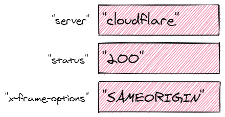
• Quick summary: unordered collection that maps keys to values using hashing.
• Also known as: hash, hash map, map, unordered map, dictionary, associative array.
• Important facts:
  • Stores data as key-value pairs.
  • Can be seen as an evolution of arrays that removes the limitation of sequential numerical indices and allows using flexible keys instead.
  • For any given non-numeric key, hashing helps get a numeric index to look up in the underlying array.
  • If hashing two or more keys returns the same value, this is called a hash collision. To mitigate this, instead of storing actual values, the underlying array may hold references to linked lists that, in turn, contain all values with the same hash.
  • A set is a variation of a hash table that stores keys but not values.
• Pros:
  • Keys can be of many data types. The only requirement is that these data types are hashable.
  • Average search, insertion and deletion are O(1).
• Cons:
  • Worst-case lookups are O(n).
  • No ordering means looking up minimum and maximum values is expensive.
  • Looking up the value for a given key can be done in constant time, but looking up the keys for a given value is O(n).
• Notable uses:
  • Caching.
  • Database partitioning.
• Time complexity (worst case):
  • Access: O(n)
  • Search: O(n)
  • Insertion: O(n)
  • Deletion: O(n)
• See also:
  • Interview Problems: Hash Maps

xxxxxxxxxx

print("Bob: " + phone_book.retrieve("Bob"))

class SimpleHashMap:

    def __init__(self):

        self.capacity = 10

        self.table = [None] * self.capacity

​

    def _hash_key(self, key):

        hash_val = 0

        for char in str(key):

            hash_val += ord(char)

        return hash_val % self.capacity

​

    def insert(self, key, value):

        hash_index = self._hash_key(key)

        key_value_pair = [key, value]

​

        if self.table[hash_index] is None:

            self.table[hash_index] = [key_value_pair]

            return True

        else:

            for pair in self.table[hash_index]:

                if pair[0] == key:

                    pair[1] = value

                    return True

            self.table[hash_index].append(key_value_pair)

            return True

​

    def retrieve(self, key):

        hash_index = self._hash_key(key)

        if self.table[hash_index] is not None:

Graph

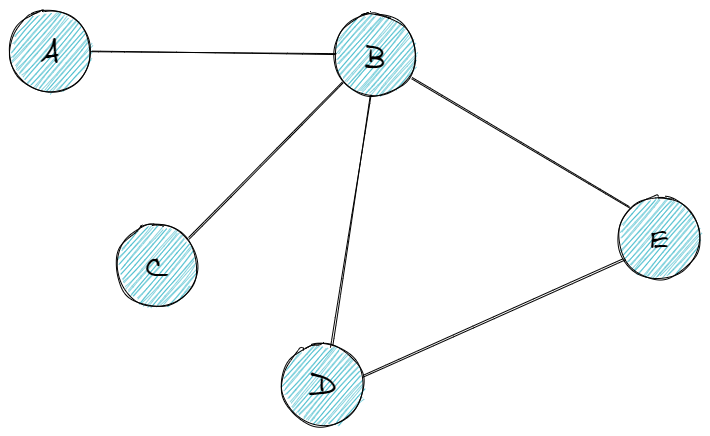
• Quick summary: a data structure that stores items in a connected, non-hierarchical network.
• Important facts:
  • Each graph element is called a node, or vertex.
  • Graph nodes are connected by edges.
  • Graphs can be directed or undirected.
  • Graphs can be cyclic or acyclic. A cyclic graph contains a path from at least one node back to itself.
  • Graphs can be weighted or unweighted. In a weighted graph, each edge has a certain numerical weight.
  • Graphs can be traversed. See important facts under Tree for an overview of traversal algorithms.
  • Data structures used to represent graphs:
    • Edge list: a list of all graph edges represented by pairs of nodes that these edges connect.
    • Adjacency list: a list or hash table where a key represents a node and its value represents the list of this node's neighbors.
    • Adjacency matrix: a matrix of binary values indicating whether any two nodes are connected.
• Pros:
  • Ideal for representing entities interconnected with links.
• Cons:
  • Low performance makes scaling hard.
• Notable uses:
  • Social media networks.
  • Recommendations in ecommerce websites.
  • Mapping services.
• Time complexity (worst case): varies depending on the choice of algorithm. O(n*lg(n)) or slower for most graph algorithms.
• See also:
  • The Simple Reference to Graphs

xxxxxxxxxx

    print(my_graph.node_links)

class GraphStructure:

    def __init__(self):

        self.node_links = {}

​

    def add_node(self, node_label):

        self.node_links[node_label] = []

​

    def connect_nodes(self, node1, node2):

        self.node_links[node1].append(node2)

        self.node_links[node2].append(node1)

​

    def remove_node(self, node):

        if node in self.node_links:

            del self.node_links[node]

​

        for vertex in self.node_links.values():

            vertex.remove(node) if node in vertex else None

​

    def disconnect_nodes(self, node1, node2):

        self.node_links[node1].remove(node2)

        self.node_links[node2].remove(node1)

​

if __name__ == '__main__':

    my_graph = GraphStructure()

    vertices = ["A", "B", "C", "D", "E", "F", "G"]

    for vertex in vertices:

        my_graph.add_node(vertex)

​

    my_graph.connect_nodes("A", "G")

Tree

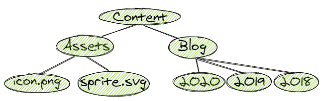
• Quick summary: a data structure that stores a hierarchy of values.
• Important facts:
  • Organizes values hierarchically.
  • A tree item is called a node, and every node is connected to 0 or more child nodes using links.
  • A tree is a kind of graph where between any two nodes, there is only one possible path.
  • The top node in a tree that has no parent nodes is called the root.
  • Nodes that have no children are called leaves.
  • The number of links from the root to a node is called that node's depth.
  • The height of a tree is the number of links from its root to the furthest leaf.
  • In a binary tree, nodes cannot have more than two children.
    • Any node can have one left and one right child node.
    • Used to make binary search trees.
    • In an unbalanced binary tree, there is a significant difference in height between subtrees.
    • An completely one-sided tree is called a degenerate tree and becomes equivalent to a linked list.
  • Trees (and graphs in general) can be traversed in several ways:
    • Breadth first search (BFS): nodes one link away from the root are visited first, then nodes two links away, etc. BFS finds the shortest path between the starting node and any other reachable node.
    • Depth first search (DFS): nodes are visited as deep as possible down the leftmost path, then by the next path to the right, etc. This method is less memory intensive than BFS. It comes in several flavors, including:
      • Pre order traversal (similar to DFS): after the current node, the left subtree is visited, then the right subtree.
      • In order traversal: the left subtree is visited first, then the current node, then the right subtree.
      • Post order traversal. the left subtree is visited first, then the right subtree, and finally the current node.
• Pros:
  • For most operations, the average time complexity is O(log(n)), which enables solid scalability. Worst time complexity varies between O(log(n)) and O(n).
• Cons:
  • Performance degrades as trees lose balance, and re-balancing requires effort.
  • No constant time operations: trees are moderately fast at everything they do.
• Notable uses:
  • File systems.
  • Database indexing.
  • Syntax trees.
  • Comment threads.
• Time complexity: varies for different kinds of trees.
• See also:
  • Interview Problems: Trees

xxxxxxxxxx

print(children[1].get_parent_node())

class TreeNode:

    def __init__(self, value):

        self.value = value

        self.children = []

        self.parent = None

​

    def set_parent_node(self, node):

        self.parent = node

​

    def get_parent_node(self):

        return self.parent

​

    def add_node(self, node):

        node.set_parent_node(self)

        self.children.append(node)

​

    def get_children(self):

        return self.children

​

    def remove_children(self):

        self.children = []

​

​

root = TreeNode(1)

root.add_node(TreeNode(2))

root.add_node(TreeNode(3))

​

children = root.get_children()

for i in range(len(children)):

Binary Search Tree

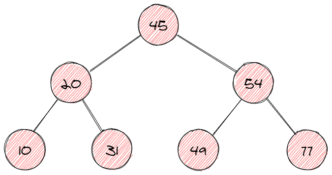
• Quick summary: a kind of binary tree where nodes to the left are smaller, and nodes to the right are larger than the current node.
• Important facts:
  • Nodes of a binary search tree (BST) are ordered in a specific way:
    • All nodes to the left of the current node are smaller (or sometimes smaller or equal) than the current node.
    • All nodes to the right of the current node are larger than the current node.
  • Duplicate nodes are usually not allowed.
• Pros:
  • Balanced BSTs are moderately performant for all operations.
  • Since BST is sorted, reading its nodes in sorted order can be done in O(n), and search for a node closest to a value can be done in O(log(n))
• Cons:
  • Same as trees in general: no constant time operations, performance degradation in unbalanced trees.
• Time complexity (worst case):
  • Access: O(n)
  • Search: O(n)
  • Insertion: O(n)
  • Deletion: O(n)
• Time complexity (average case):
  • Access: O(log(n))
  • Search: O(log(n))
  • Insertion: O(log(n))
  • Deletion: O(log(n))
• See also:
  • An Intro to Binary Trees and Binary Search Trees
  • Interview Problems: Binary Search Trees

xxxxxxxxxx

    tree.preorder()

class Node(object):

    def __init__(self, val):

        self.val = val

        self.left_child = None

        self.right_child = None

​

    def insert(self, val):

        """For inserting the value in the Tree"""

        if self.val == val:

            return False  # A BST cannot contain duplicate data

​

        elif val < self.val:

            """Values less than the root data are placed to the left of the root"""

            if self.left_child:

                return self.left_child.insert(val)

            else:

                self.left_child = Node(val)

                return True

​

        else:

            """Values greater than the root data are placed to the right of the root"""

            if self.right_child:

                return self.right_child.insert(val)

            else:

                self.right_child = Node(val)

                return True

​

    def min_node(self, node):

        current = node