

Dynamic programming is a technique for solving problems, whose solution can be expressed recursively in terms of solutions of overlapping sub-problems. A gentle introduction to this can be found in How Does DP Work? Dynamic Programming Tutorial.
Memoization is an optimization process. In simple terms, we store the intermediate results of the solutions of sub-problems, allowing us to speed up the computation of the overall solution. The improvement can be reduced to an exponential time solution to a polynomial time solution, with an overhead of using additional memory for storing intermediate results.
Let's understand how dynamic programming works with memoization with a simple example.
Introduction to Fibonacci Numbers
The enigmatic Fibonacci sequence: many of you have crossed paths with this numerical series before, possibly while exploring recursion. Today, we delve into how this seemingly simple sequence can serve as an excellent introduction to the powerhouses of computer science—dynamic programming and memoization.
The Mathematical Definition of Fibonacci Numbers
The Fibonacci sequence is mathematically defined as follows:
Code Snippets in Multiple Languages
To solidify your understanding, let's translate this mathematical definition into several programming languages.
1# Base case for n = 0
2if n == 0:
3    return 0
4# Base case for n = 1
5if n == 1:
6    return 1
7# Recursive case for n > 1
8return f(n-1) + f(n-2)
Sequence Unveiled
By applying the above code, you'll generate a sequence like so:
10, 1, 1, 2, 3, 5, 8, 13, 21, 34, ...Pseudocode: The Blueprint of Fibonacci
Pseudocode is a programmer's sketchbook. It helps you outline your logic before jumping into the code. For the Fibonacci sequence, our pseudocode would look something like this:
Base Case
- If , return 0.
- If , return 1.
Recursive Case
- Calculate and store it in
temp1. - Calculate and store it in
temp2. - Return
temp1 + temp2.
xxxxxxxxxxdef f(n): if n==0: return 0 if n==1: return 1 temp1 = f(n-1) temp2 = f(n-2) return temp1 + temp2Analyzing the Recursion Tree: Uncovering the Achilles' Heel
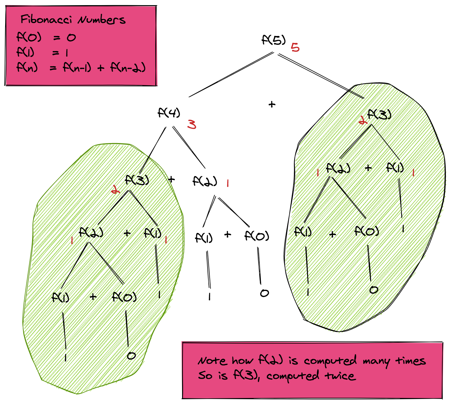
You've seen how the Fibonacci sequence works; now let's peek under the hood. Imagine the Fibonacci sequence as a sprawling tree, where each branch splits into smaller branches until you reach the leaves, which are the base cases.
The Problem of Redundancy
If you study the recursion tree for calculating , you'll notice something disconcerting. Multiple nodes represent the same Fibonacci number! For example, is computed twice, is calculated thrice, and the base cases and appear even more frequently.
Time Complexity: It's Exponential!
Because of this redundancy, our naive recursive approach has a time complexity of . In non-mathematical terms, that means it's slow, especially for larger values of .
The Power of Memoization
Here's the good news: we don't have to live with this inefficiency. By storing the results of computations we've already done, we can avoid redundant calculations. This technique is called memoization, and it's a cornerstone of dynamic programming.
The Road to Optimization
Memoization is like a cheat sheet for your algorithm. It's a simple yet powerful way to remember past results, so you don't have to recalculate them. Here's how it generally works:
Steps to Implement Memoization
- Create a data structure (usually an array or hash table) to store computed values.
- Before diving into the recursive calls, check if the result for the current is already in the storage.
- If it is, use that value instead of making a new recursive call.
- If not, proceed with the recursion and store the new result in the data structure.
By doing this, you can dramatically reduce the time complexity from exponential to linear, i.e., .
Memoization of Fibonacci Numbers: From Exponential Time Complexity to Linear Time Complexity
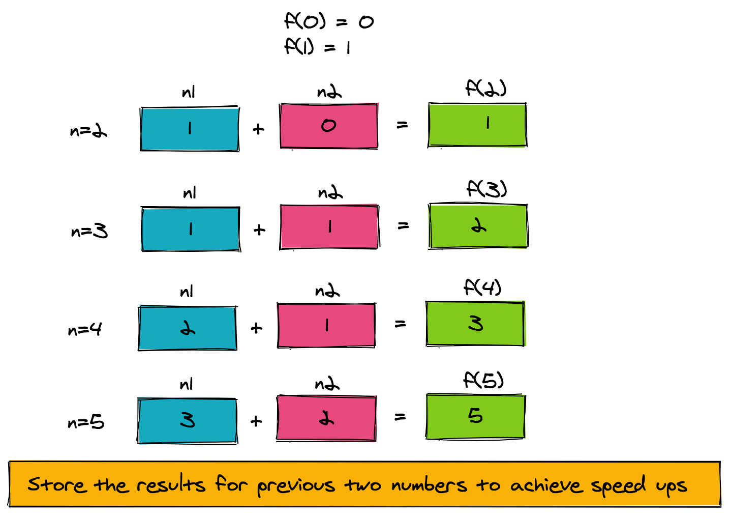
To speed things up, let's look at the structure of the problem. f(n) is computed from f(n-1) and f(n-2). As such, we only need to store the intermediate result of the function computed for the previous two numbers. The pseudo-code to achieve this is provided here.
The figure below shows how the pseudo-code is working for f(5). Notice how a very simple memoization technique that uses two extra memory slots has reduced our time complexity from exponential to linear (O(n)).
1Routine: fibonacciFast
2Input: n
3Output: Fibonacci number at the nth place
4Intermediate storage: n1, n2 to store f(n-1) and f(n-2) respectively
5
61. if (n==0) return 0
72. if (n==1) return 1
83. n1 = 1
94. n2 = 0
105. for 2 .. n
11    a. result = n1+n2           // gives f(n)
12    b.   n2 = n1                // set up f(n-2) for next number
13    c.   n1 = result            // set up f(n-1) for next number
146. return resultxxxxxxxxxxdef fibonacciFast(n): if (n == 0): return 0 if (n == 1): return 1 n1 = 1 n2 = 0 result = 0 for i in range(2, n + 1): result = n1 + n2 # gives f(n) n2 = n1 # set up f(n-2) for next number n1 = result # set up f(n-1) for next number return resultprint(fibonacciFast(10))Build your intuition. Is this statement true or false?
Dynamic programming problems have the property of having optimal solutions and overlapping sub-problems.
Press true if you believe the statement is correct, or false otherwise.
From Naive to Smart: Maximizing Grid Rewards
Ah, the grid! Picture it as a treasure map where each cell has its own hidden gem (or, let's say, reward). Our trusty robot wants to navigate this map to find the ultimate treasure—the maximum reward. But there's a catch! The robot can only move up or to the right. How do we make sure our robotic friend picks the richest path?
The Brute-Force Way: Recursive Enumeration
If you've read the tutorial on recursion and backtracking, you know that you can enumerate all paths using backtracking. It's like the robot taking a stroll, noting down each path and the rewards it accumulates.
Steps for Recursive Enumeration
- Walk through all possible paths while keeping track of the reward for each path.
- Select the path that garners the maximum reward.
The Downside: Exponential Complexity
This might sound like a simple plan, but it's a costly one. Just like our previous Fibonacci example, this naive approach has an exponential time complexity of . That's a lot of calculations, and our robot doesn't have all day!
Enter Dynamic Programming: A Smarter Approach
Let's switch gears and bring dynamic programming into the picture. Just like we did with the Fibonacci numbers, we can avoid recalculating rewards for the same cell multiple times. This is how dynamic programming turns our robot into a strategic treasure hunter.
Steps to Implement Dynamic Programming
- Create a 2D array,
dp, with dimensions (m \times n). - Initialize
dp[0][0]with the reward of the starting cell. - Loop through the grid, and for each cell
(i, j), updatedp[i][j]as the maximum reward you can get by either coming from the top celldp[i-1][j]or the left celldp[i][j-1], plus the reward at(i, j). - The value at
dp[m-1][n-1]will be the maximum reward.
By following these steps, we reduce our time complexity from exponential to linear, , which is a significant improvement.
Path Finding with Dynamic Programming
Let's take a step back.
Imagine you're navigating a maze, and each cell in the maze offers you a reward. Your aim is to find the path from the starting point to the destination that maximizes these rewards. This is like a treasure hunt, except you're gathering coins or gems along the way.
The Aha Moment: A Single Principle
Let's crystallize our approach with a powerful observation:
If the richest path passes through a cell at
(r, c), then the path leading up to(r, c)and the path leading away from(r, c)to the goal must also be the richest.
Picture it as a road trip where you have multiple stops. If a city along your route is the richest in terms of tourist attractions, the route to that city and beyond must also offer the most attractions.
Breaking Down the Problem
We've essentially divided a big challenge into two smaller tasks:
- Finding the Richest Path to
(r, c): What's the best route from the start to this cell? - Finding the Richest Path from
(r, c)to Goal: What's the best route from this cell to the destination?
Combine these, and voila, you have your ultimate treasure-rich path.
The Role of Memoization
Just like you'd mark checkpoints on a map, we'll mark the richest path to each cell in a matrix called reward. This matrix will store the maximum accumulated reward from the starting cell to every other cell on the grid.
Two Key Matrices
- Input Matrix : This holds the reward for each individual cell at
(r, c). - Memoization Matrix : This stores the maximum accumulated reward from the start to each cell
(r, c).
Think of the first matrix as the list of tourist attractions in each city, and the second matrix as your travel diary, recording the best experiences up to each point.
By the end of this exercise, the cell in reward corresponding to the goal will hold the maximum reward possible. Just follow the path back, and you've solved the maze in the most rewarding way.
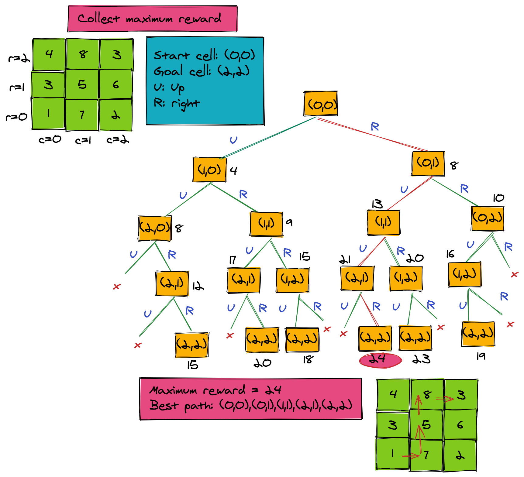
Here is the recursive pseudo-code that finds the maximum reward from the start to the goal cell. The pseudo-code finds the maximum possible reward when moving up or right on an m x n grid. Let's assume that the start cell is (0, 0) and the goal cell is (m-1, n-1).
To get an understanding of the working of this algorithm, look at the figure below. It shows the maximum possible reward that can be collected when moving from start cell to any cell. For now, ignore the direction matrix in red.
1Routine: maximizeReward
2Start cell coordinates: (0, 0)
3Goal cell coordinates: (m-1, n-1)
4Input: Reward matrix w of dimensions mxn
5
6Base case 1:
7// for cell[0, 0]
8reward[0, 0] = w[0, 0]
9
10Base case 2:
11// zeroth col.  Can only move up
12reward[r, 0] = reward[r-1, 0] + w[r, 0]  for r=1..m-1
13
14Base case 3:
15// zeroth row.  Can only move right
16reward[0,c] = reward[0, c-1] + w[0, c] for c=1..n-1
17
18Recursive case:
191. for r=1..m-1
20    a. for c=1..n-1
21        i. reward[r,c] = max(reward[r-1, c],reward[r, c-1]) + w[r, c]
222. return reward[m-1, n-1]           // maximum reward at goal state
Finding the Path via Memoization
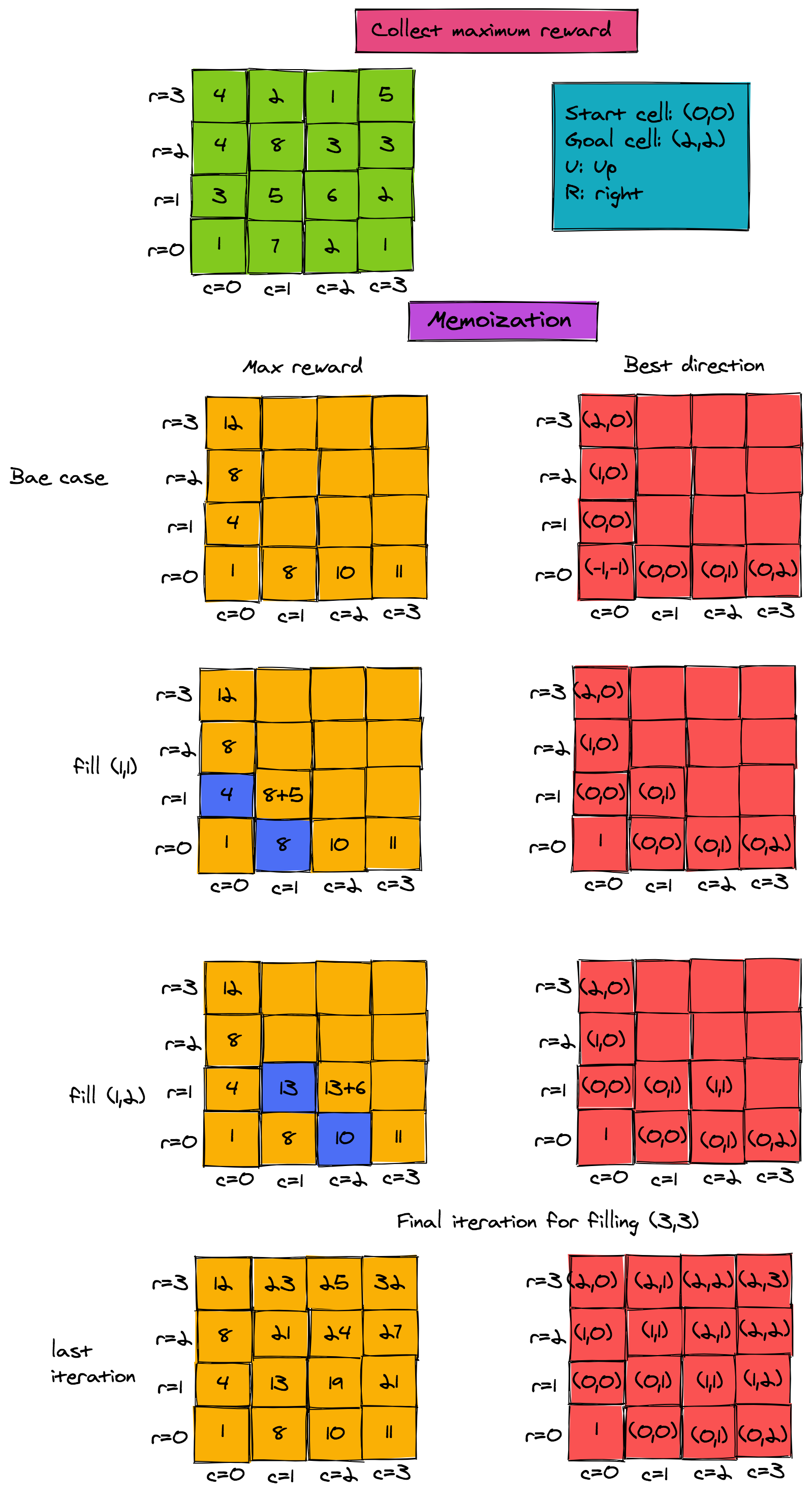
Finding the actual path is also easy. All we need is an additional matrix, which stores the predecessor for each cell (r, c) when finding the maximum path. For example, in the figure above, when filling (1, 1), the maximum reward would be 8+5 when the predecessor in the path is the cell (0, 1). We need one additional matrix d that gives us the direction of the predecessor:
1d[r,c] = coordinates of the predecessor in the optimal path reaching `[r, c]`. Here is the translation:
1# d[r,c] = coordinates of the predecessor in the optimal path reaching `[r, c]`.The pseudo-code for filling the direction matrix is given by the attached pseudocode.
1Routine: bestDirection
2routine will fill up the direction matrix
3Start cell coordinates: (0,0)
4Goal cell coordinates: (m-1,n-1)
5Input: Reward matrix w
6
7Base case 1:
8// for cell[0,0]
9d[0,0] = (-1, -1)      //not used
10
11Base case 2:
12// zeroth col.  Can only move up
13d[r,0] = (r-1, 0)   for r=1..m-1
14
15Base case 3:
16// zeroth row.  Can only move right
17reward[0, c] = d[0,c-1] for c=1..n-1
18
19Recursive case:
201. for r=1..m-1
21    a. for c=1..n-1
22        i. if reward[r-1,c] > reward[r,c-1])
23                then d[r,c] = (r-1, c)
24           else
25                 d[r,c] = (r, c-1)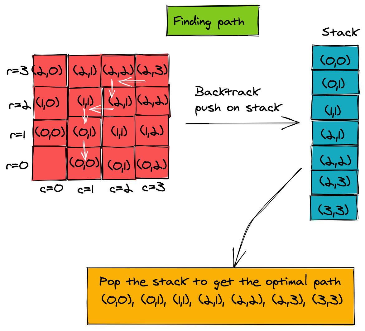
262. return dxxxxxxxxxxreturn d;// Routine: bestDirection// Routine will fill up the direction matrix// Start cell coordinates: (0,0)// Goal cell coordinates: (m-1,n-1)// Input: Reward matrix w// Base case 1:// For cell[0,0]d[0,0] = new int[] {-1, -1}; //not used// Base case 2:// Zeroth col. Can only move upfor (int r=1; r<m; r++) d[r,0] = new int[] {r-1, 0};// Base case 3:// Zeroth row. Can only move rightfor (int c=1; c<n; c++) d[0,c] = d[0,c-1];// Recursive case:for (int r=1; r<m; r++) { for (int c=1; c<n; c++) { if (w[r-1,c] > w[r,c-1]) d[r,c] = new int[] {r-1, c}; else d[r,c] = new int[] {r, c-1}; }}Once we have the direction matrix, we can backtrack to find the best path, starting from the goal cell (m-1, n-1). Each cell's predecessor is stored in the matrix d.
If we follow this chain of predecessors, we can continue until we reach the start cell (0, 0). Of course, this means we'll get the path elements in the reverse direction. To solve for this, we can push each item of the path on a stack and pop them to get the final path. The steps taken by the pseudo-code are shown in the figure below.
1Routine: printPath
2Input: direction matrix d
3Intermediate storage: stack
4
5// build the stack
61. r = m-1
72. c = n-1
83. push (r, c) on stack
94. while (r!=0 && c!=0)
10    a. (r, c) = d[r, c]
11    b. push (r, c) on stack
12// print final path by popping stack
135. while (stack is not empty)
14    a. (r, c) = stack_top
15    b. print (r, c)
16 c. pop_stackxxxxxxxxxxstack = []r = m - 1c = n - 1stack.append((r, c))while r != 0 and c != 0: r, c = d[r][c] stack.append((r, c))while stack: r, c = stack[-1] print(f"({r}, {c})") stack.pop()Time Complexity of Path Using Dynamic Programming and Memoization
We can see that using matrices for intermediate storage drastically reduces the computation time. The maximizeReward function fills each cell of the matrix only once, so its time complexity is O(m * n). Similarly, the best direction also has a time complexity of O(m * n).
The printPath routine would print the entire path in O(m+n) time. Thus, the overall time complexity of this path finding algorithm is O(m * n). This means we have a drastic reduction in time complexity from O(2) to O(m + n). This, of course, comes at a cost of additional storage. We need additional reward and direction matrices of size m * n, making the space complexity O(m * n). The stack of course uses O(m+n) space, so the overall space complexity is O(m * n).
Build your intuition. Fill in the missing part by typing it in.
Applying memoization to a problem increases _ complexity, and decreases _ complexity.
(Please write your answer as a comma separated string)
Write the missing line below.
Weighted Interval Scheduling via Dynamic Programming and Memoization
Our last example in exploring the use of memoization and dynamic programming is the weighted interval scheduling problem.
We are given n intervals, each having a start and finish time, and a weight associated with them. Some sets of intervals overlap and some sets do not. The goal is to find a set of non-overlapping intervals to maximize the total weight of the selected intervals. This is a very interesting problem in computer science, as it is used in scheduling CPU tasks, and in manufacturing units to maximize profits and minimize costs.
Problem Parameters
The following are the parameters of the problem:
11. n = total intervals. We'll use an additional zeroth interval for base case.
22. Each interval has a start time and a finish time.
3 Hence there are two arrays s and f, both of size (n+1)
4 s[j] < f[j] for j=1..n and s[0] = f[0] = 0
53. Each interval has a weight w, so we have a weight array w. w[j] >0 for j=1..n and w[0]=0
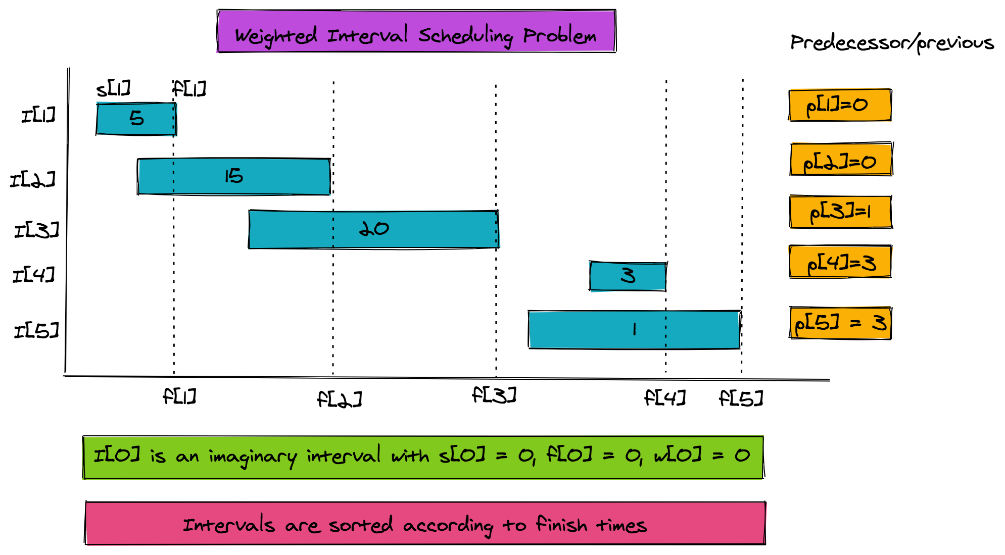
64. The interval array is sorted according to finish times.Additionally we need a predecessor array p:
16. p[j] = The non-overlapping interval with highest finish time which is less than f[j].
2            p[j] is the interval that finishes before p[j]
To find p[j], we only look to the left for the first non-overlapping interval. The figure below shows all the problem parameters.
A Recursive Expression for Weighted Interval Scheduling
As mentioned before, dynamic programming combines the solutions of overlapping sub-problems. Such a problem, the interval scheduling for collecting maximum weights, is relatively easy.
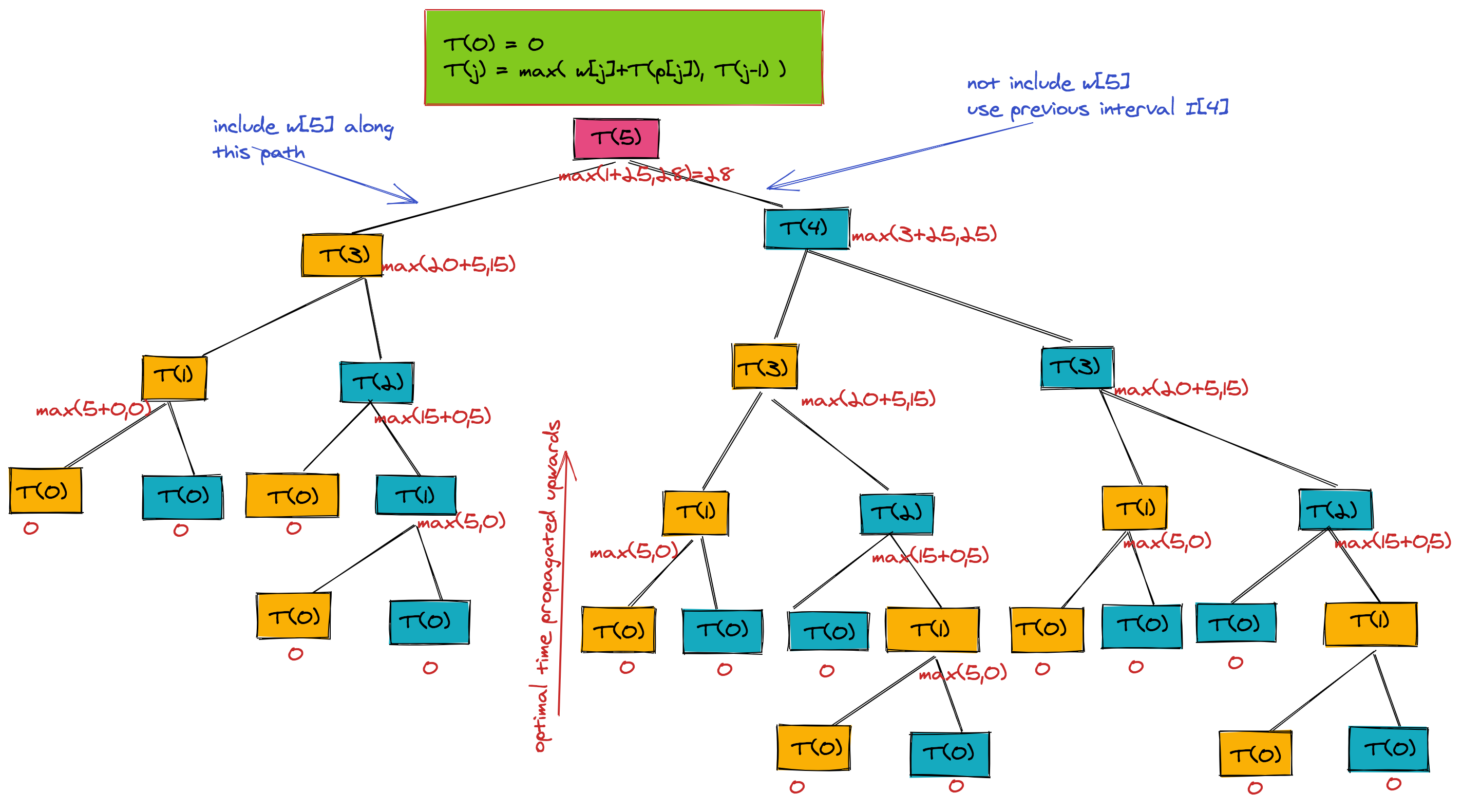
For any interval j, the maximum weight can be computed by either including it or excluding it. If we include it, then we can compute the sum of weights for p[j], as p[j] is the first non-overlapping interval that finishes before I[j]. If we exclude it, then we can start looking at intervals j-1 and lower. The attached is the recursive mathematical formulation.
The below figure shows the recursion tree when T(5) is run.
1Routine: T(j)
2Input: s, f and w arrays (indices 0..n).  Intervals are sorted according to finish times
3Output: Maximum accumulated weight of non-overlapping intervals
4
5Base case:
61. if j==0 return 0
7
8Recursive case T(j):
91. T1 = w[j] + T(p[j])
102. T2 = T(j-1)
113. return max(T1,T2)xxxxxxxxxx# Routine: T(j)# Input: s, f and w arrays (indices 0..n). Intervals are sorted according to finish times# Output: Maximum accumulated weight of non-overlapping intervals# Base case:if j == 0: return 0# Recursive case T(j):T1 = w[j] + T(p[j])T2 = T(j - 1)return max(T1, T2)Scheduling via Dynamic Programming and Memoization
From the recursion tree, we can see that the pseudo-code for running the T function has an exponential time complexity of O(2). From the tree, we can see how to optimize our code. There are parameter values for which T is computed more than once-- examples being T(2), T(3), etc. We can make it more efficient by storing all intermediate results and using those results when needed, rather than computing them again and again. Here's the faster version of the pseudo-code, while using an additional array M for memoization of maximum weights up to nth interval.
1# Routine: TFast(j)
2# Input: f, s and w arrays (indices 0..n). Intervals sorted according to finish times
3# Output: Maximum accumulated weight of non-overlapping intervals
4# Intermediate storage: Array M size (n+1) initialized to -1
5def TFast(j):
6    # Base case:
7    if j == 0:
8        M[0] = 0
9        return 0
10
11    # Recursive case:
12    if M[j] != -1:        # if result is stored
13        return M[j]       # return the stored result
14
15    T1 = w[j] + TFast(p[j])
16    T2 = TFast(j-1)
17    M[j] = max(T1, T2)
18
19    return M[j]
`
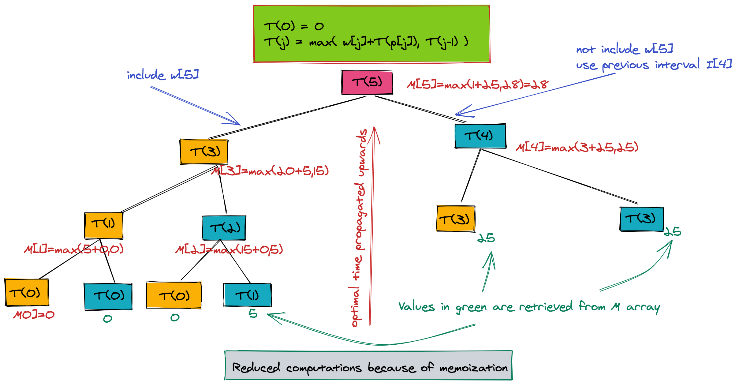
The great thing about this code is that it would only compute TFast for the required values of j. The tree below is the reduced tree when using memoization. The values are still propagated from leaf to root, but there is a drastic reduction in the size of this tree.
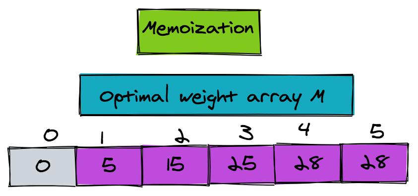
The figure shows the optimal weight array M:
Finding the Interval Set
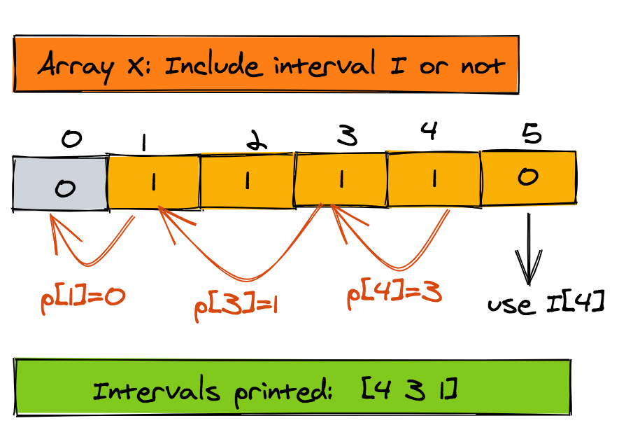
There is one thing left to do-- find out which intervals make up the optimal set. We can use an additional array X, which is a Boolean array. X[j] indicates whether we included or excluded the interval j, when computing the max. We can fill up array X as we fill up array M. Let's change TFast to a new function TFastX to do just that.
We can retrieve the interval set using the predecessor array p and the X array. Below is the pseudo-code:
1j = n
2while j > 0:
3    if X[j] == 1: #Is j to be included?
4        print(j)
5        j = p[j] #get predecessor of j
6    else:
7        j = j - 1
The whole process is illustrated nicely in the figure below. Note in this case too, the intervals are printed in descending order according to their finish times. If you want them printed in reverse, then use a stack like we did in the grid navigation problem. That change should be trivial to make.
1Routine: TFastX(j)
2Input: f,s and w arrays (indices 0..n).  Intervals sorted according to finish times
3Output: Maximum accumulated weight of non-overlapping intervals
4Intermediate storage: Array M size (n+1) initialized to -1,
5                      Array X size (n+1) initialized to 0
6
7Base case:
81. if j==0
9M[0] = 0;
10X[0] = 0
11return 0
12
13Recursive case TfastX(j):
141. if M[j] != -1            // if result is stored
15return M[j]                 // return the stored result
161. T1 = w[j] + TFast[p[j]]
172. T2 = TFast[j-1]
183. if (T1 > T2)
19        X[j] = 1                    // include jth interval else X[j] remains 0
204. M[j] = max(T1, T2)
215. return M[j]xxxxxxxxxx# Python Implementationdef TFastX(j, w, p, M, X): if j == 0: M[0] = 0 X[0] = 0 return 0 if M[j] != -1: return M[j] T1 = w[j] + TFastX(p[j], w, p, M, X) T2 = TFastX(j-1, w, p, M, X) if T1 > T2: X[j] = 1 M[j] = max(T1, T2) return M[j]Time Complexity of Weighted Interval Scheduling via Memoization
The time complexity of the memoized version is O(n). It is easy to see that each slot in the array is filled only once. For each element of the array, there are only two values to choose the maximum from-- thus the overall time complexity is O(n). However, we assume that the intervals are already sorted according to their finish times. If we have unsorted intervals, then there is an additional overhead of sorting the intervals, which would require O(n log n) computations.
Well, that's it for now. You can look at the Coin Change problem and Longest Increasing Subsequence for more examples of dynamic programming. I hope you enjoyed this tutorial as much as I did creating it!
Build your intuition. Click the correct answer from the options.
Solving Longest Increasing Subsequence problem using dynamic programming with memoization will have the time complexity:
Click the option that best answers the question.
- O(n)
- O(n^2)
- O(log n)
- O(n log n)
Try this exercise. Fill in the missing part by typing it in.
Solving Longest Increasing Subsequence problem using dynamic programming with memoization will have the space complexity ____.
Write the missing line below.
One Pager Cheat Sheet
Dynamic Programming (DP) with Memoization is a technique for optimizing the solution of overlapping sub-problems to anexponential time solutionto apolynomial time solution, while using additional memory to store intermediate results.- This sentence summarizes the concept of Fibonacci Numbers, which is defined and implemented utilizing a recursive design pattern, wherein each number is the sum of the two preceding numbers
in the sequence. - By examining the recursion tree for computing
fibonacci(5), we can deduce an exponentialO(2^n)complexity, with potential for speedups by using stored intermediate results. - We can reduce the exponential time complexity of our Fibonacci computation from
O(2^n)toO(n)using a simplememoizationtechnique with only two extra memory spaces. - Dynamic Programming (DP) is a powerful algorithmic technique used to efficiently solve problems with optimal solutions and overlapping sub-problems through
memoization, reducing the complexity from exponential (O(n^2)) to linear (O(n)). - Finding the path with the highest reward through an
m * ngrid usingBacktrackingrequires enumerating all possible paths and selecting the one with the maximum reward, resulting in an exponential time complexity of O(2). - By combining the technique of Dynamic Programming with the Memoization of accumulated rewards stored in the
rewardmatrix, we can find the optimum, or best, path from the start to goal that collects the maximum reward. - The pseudo-code finds the maximum reward when moving up or right on a
m x ngrid, from(0, 0)to(m-1, n-1). - The
optimal pathto a maximum reward can be found by filling an additional matrixdwhich stores thepredecessorfor each cell(r, c)when finding themaximum path. - We can use the
direction matrixtobacktrackfrom the goal cell to the start cell andpopthe elements off a stack to get the final path. - Using Dynamic Programming and Memoization, we can drastically reduce the time complexity from O(2) to
O(m * n), but with acost of additional storageofO(m * n)space complexity. - Memoization is a
techniquewhich increases space complexity but drastically reduces time complexity, allowing for a significantly faster algorithm. - The
problem parametersgiven allow us to usedynamic programmingandmemoizationto solve the weighted interval scheduling problem in order tomaximizethe total weight of thenon-overlappingintervals. - A maximum weight for an interval can be computed recursively by either including or excluding it, and looking at the intervals
j-1and lower for exclusion. - By using
Memoization, we can drastically reduce time complexity and optimize the code efficiency ofDynamic Programmingfor Scheduling. - We can
retrieve theinterval setusing thepredecessor arraypand theBoolean arrayX`. - The time complexity of the Memoized version of Weighted Interval Scheduling is
O(n), assuming the intervals are already sorted according to their finish times. - The Longest Increasing Subsequence (LIS) problem using dynamic programming with memoization has a time complexity of O(n^2), achieved by
two nested loops of O(n)computations for each of thenslots. - The space complexity of solving the Longest Increasing Subsequence (LIS) problem using dynamic programming with memoization is O(n).