

Anomaly Detection using Python
In this example we will be using a dataset which contains details of the closing prices for S&P 500 index from 1986 to 2018.
We are going to create a Long Short-Term Memory Network (LSTM) Model.
Step 1: Import Libraries
1import numpy as np
2import tensorflow as tf
3from tensorflow import keras
4import pandas as pd
5import seaborn as sns
6from pylab import rcParams
7import matplotlib.pyplot as plt
8from matplotlib import rc
9from pandas.plotting import register_matplotlib_converters
10from sklearn.model_selection import train_test_split
11from sklearn.preprocessing import StandardScaler
12rcParams['figure.figsize'] = 22, 10
13
14RANDOM_SEED = 42
15np.random.seed(RANDOM_SEED)
16tf.random.set_seed(RANDOM_SEED)
Step 2: Upload the Dataset
In this example we will be using a dataset that can be downloaded from Kaggle.
1anomaly_df = pd.read_csv('/content/spx.csv', parse_dates=['date'], index_col='date')Step 3: Manual Anomaly Detection
1fig = plt.figure()
2plt.style.use('ggplot')
3
4ax = fig.add_subplot()
5
6ax.plot(anomaly_df, label='Close Price')
7
8ax.set_title('S&P 500 Daily Prices 1986 - 2018', fontweight = 'bold')
9
10ax.set_xlabel('Year')
11ax.set_ylabel('Dollars ($)')
12
13ax.legend()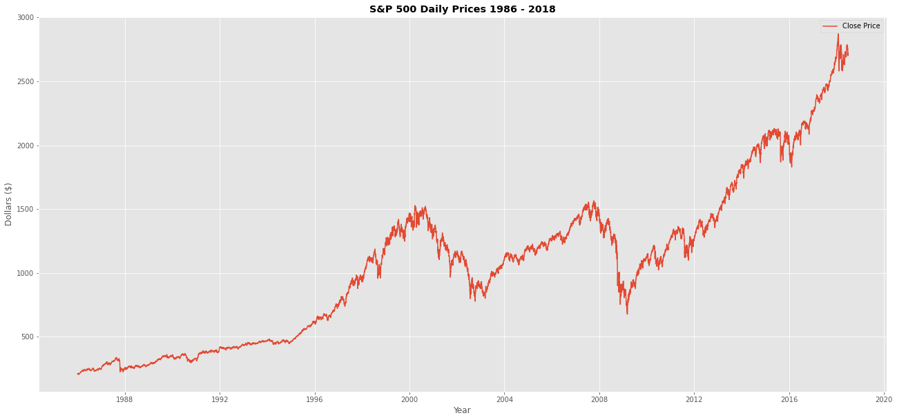
Step 4: Splitting the Dataset into Training & Testing
In this example, we are choosing to split the data into two parts:
- 95% training data, to train our machine to learn the normal patterns in the data
- 5% testing data, to evaluate the machine.
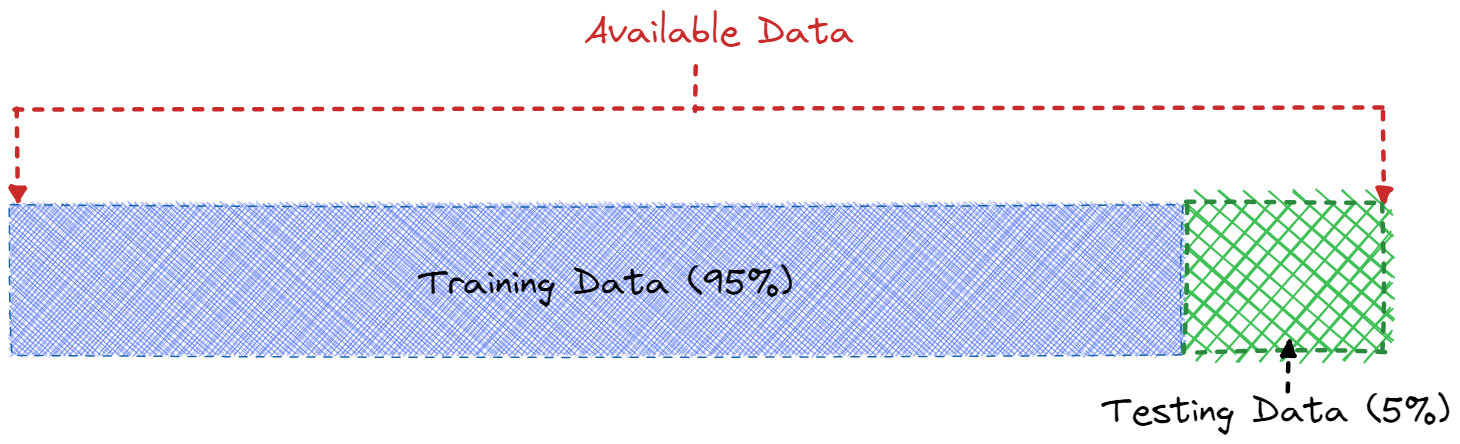
1train_size = int(len(anomaly_df) * 0.95)
2test_size = len(anomaly_df) - train_size
3train, test = anomaly_df.iloc[0:train_size], anomaly_df.iloc[train_size:len(anomaly_df)]
Step 5: Preparing the Data
First we will scale and reshape our data for the ML model.
1scaler = StandardScaler()
2scaler = scaler.fit(train[['close']])
3
4train['close'] = scaler.transform(train[['close']])
5test['close'] = scaler.transform(test[['close']])1#Create helper function
2def create_dataset(X, y, time_steps=1):
3 Xs, ys = [], []
4 for i in range(len(X) - time_steps):
5 v = X.iloc[i:(i + time_steps)].values
6 Xs.append(v)
7 ys.append(y.iloc[i + time_steps])
8 return np.array(Xs), np.array(ys)
9
10TIME_STEPS = 30
11
12# reshape to [samples, time_steps, n_features]
13
14X_train, y_train = create_dataset(train[['close']], train.close, TIME_STEPS)
15X_test, y_test = create_dataset(test[['close']], test.close, TIME_STEPS)Step 6: Create the Model
1model = keras.Sequential()
2
3#encoder
4model.add(keras.layers.LSTM(
5    units=64,
6    input_shape=(X_train.shape[1], X_train.shape[2])
7))
8model.add(keras.layers.Dropout(rate=0.2))
9
10#decoder
11model.add(keras.layers.RepeatVector(n=X_train.shape[1]))
12
13model.add(keras.layers.LSTM(units=64, return_sequences=True))
14model.add(keras.layers.Dropout(rate=0.2))
15
16model.add(keras.layers.TimeDistributed(keras.layers.Dense(units=X_train.shape[2])))
17
18model.compile(loss='mae', optimizer='adam')
19model.summary()
Step 7: Train the Model
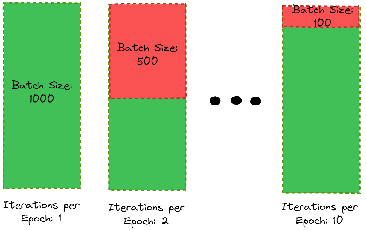
To create our model we need to decide on the most appropriate batch size and number of Epochs, changing these values will vary our models performance.
1history = model.fit(
2    X_train, y_train,
3    epochs=10,
4    batch_size=32,
5    validation_split=0.1,
6    shuffle=False
7)
To decide what is the suitable number of epochs we can visualize the result from our model.
1fig = plt.figure()
2ax = fig.add_subplot()
3
4ax.plot(history.history['loss'], label='train')
5ax.plot(history.history['val_loss'], label='test')
6
7ax.legend()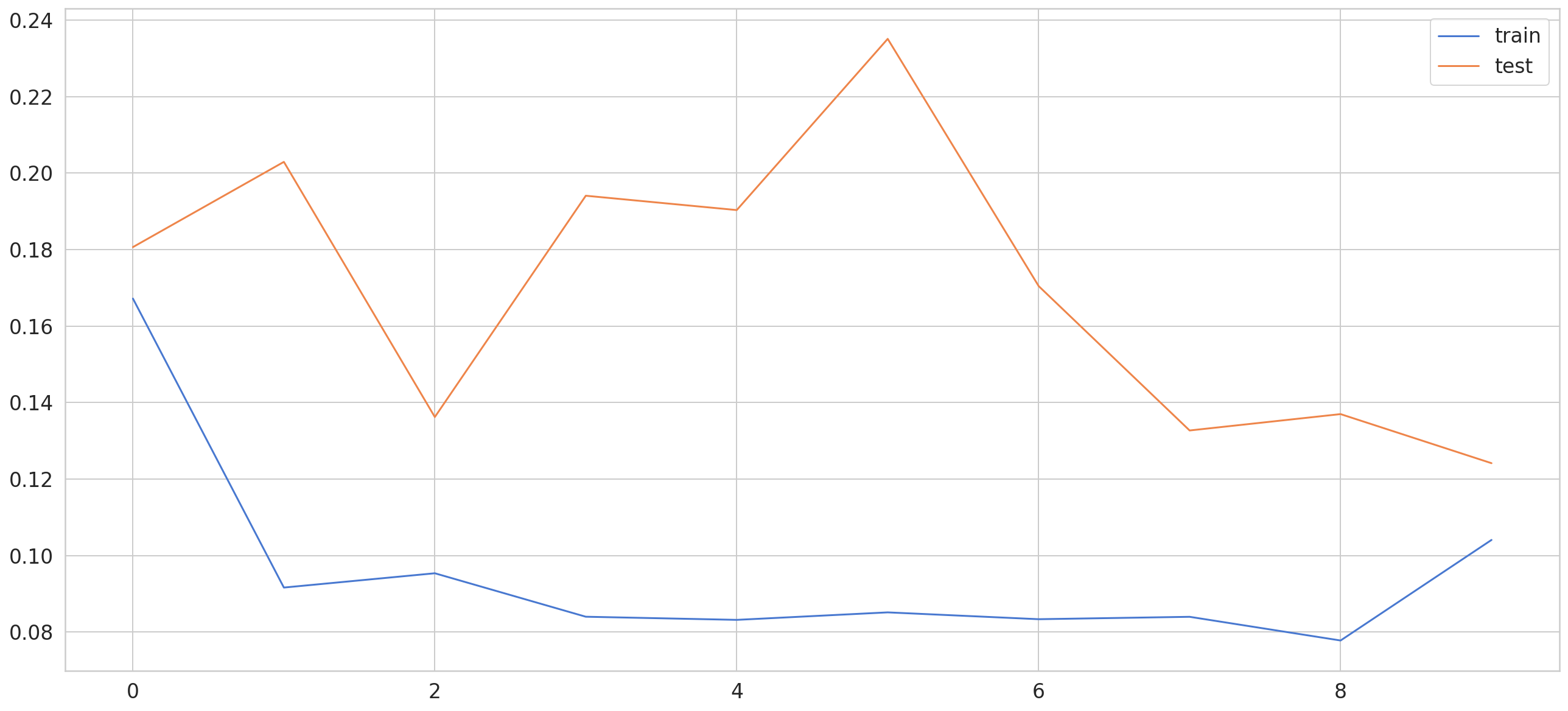
Step 8: Defining the Anomaly Value
First we will calculate the loss between the predicted and the actual closing price data:
1X_train_pred = model.predict(X_train)
2
3train_mae_loss = np.mean(np.abs(X_train_pred - X_train), axis=1)
We will then plot the loss distribution to decide on the threshold for our anomaly detection.
1fig = plt.figure(figsize=(20,10))
2sns.set(style="darkgrid")
3
4ax = fig.add_subplot()
5
6sns.distplot(train_mae_loss, bins=50, kde=True)
7
8ax.set_title('Loss Distribution Training Set ', fontweight ='bold')
Calculate the Mean Absolute Error
1X_test_pred = model.predict(X_test)
2
3test_mae_loss = np.mean(np.abs(X_test_pred - X_test), axis=1)
In this example we are using a threshold of 0.65
1THRESHOLD = 0.65
2
3test_score_df = pd.DataFrame(index=test[TIME_STEPS:].index)
4test_score_df['loss'] = test_mae_loss
5test_score_df['threshold'] = THRESHOLD
6test_score_df['anomaly'] = test_score_df.loss > test_score_df.threshold
7test_score_df['close'] = test[TIME_STEPS:].close1fig = plt.figure()
2
3ax = fig.add_subplot()
4
5ax.plot(test_score_df.index, test_score_df.loss, label='loss')
6ax.plot(test_score_df.index, test_score_df.threshold, label='threshold')
7
8ax.legend()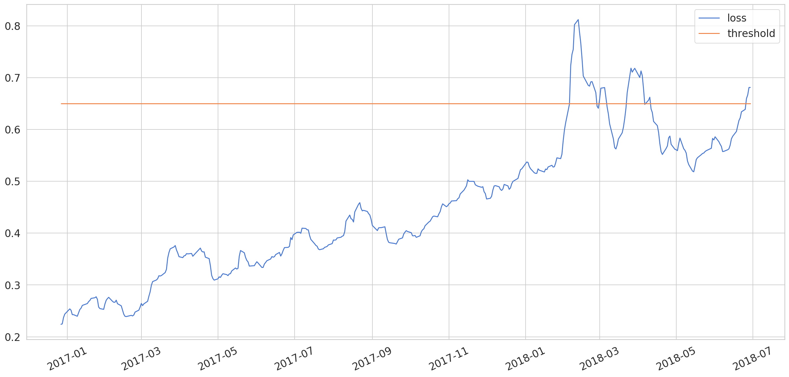
1anomalies = test_score_df[test_score_df.anomaly == True]
2anomalies.head()
And finally our anomaly detection.
1fig = plt.figure()
2
3ax = fig.add_subplot()
4
5ax.plot(test[TIME_STEPS:].index,
6  scaler.inverse_transform(test[TIME_STEPS:].close.values.reshape(1,-1)).reshape(-1),
7  label='close price')
8
9sns.scatterplot(anomalies.index, scaler.inverse_transform(anomalies.close.values.reshape(1,-1)).reshape(-1), color=sns.color_palette()[3],
10  s=52,label='anomaly')
11
12ax.legend()
We can change our anomaly threshold which will enable our model to detect more or less anomalies depending on your businesses criteria.