

Univariate Analysis
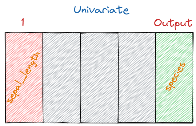
Let’s start with the simplest form of analyzing data, univariate analysis. “Uni” meaning “one,” means that we are only analyzing one feature of our dataset. Based on the one selected feature 'sepal_length', we will try to determine the output species .
PYTHON
1# Import libraries
2import pandas as pd
3import numpy as np
4import matplotlib.pyplot as plt
5import seaborn as sns
6
7# Import the dataset
8df = sns.load_dataset('iris')
First we are dividing out data frame up into three separate data frames for each category.
PYTHON
1setosa_filter = df['species'] == 'setosa'
2virginica_filter = df['species'] == 'virginica'
3versicolor_filter = df['species'] == 'versicolor'
4
5setosa_df = df.loc[setosa_filter,:]
6virginica_df = df.loc[virginica_filter,:]
7versicolor_df = df.loc[versicolor_filter,:]
Next we will plot the feature, since this is a univariate analysis we make everything on the Y axis equal to zero.
PYTHON
1plt.plot(setosa_df['sepal_length'],np.zeros_like(setosa_df['sepal_length']),'o')
2plt.plot(virginica_df['sepal_length'],np.zeros_like(virginica_df['sepal_length']),'o')
3plt.plot(versicolor_df['sepal_length'],np.zeros_like(versicolor_df['sepal_length']),'o')
4plt.xlabel('Sepal length', fontweight = 'bold')
5plt.show()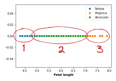
As you can see from our plot it is quite easy to find the ranges and distinguish which category each data point falls into by their petal length.